A Framework for Quantum Finite-State Languages with Density Mapping
Abstract
A quantum finite-state automaton (QFA) is a theoretical model designed to simulate the evolution of a quantum system with finite memory in response to sequential input strings. We define the language of a QFA as the set of strings that lead the QFA to an accepting state when processed from its initial state. QFAs exemplify how quantum computing can achieve greater efficiency compared to classical computing. While being one of the simplest quantum models, QFAs are still notably challenging to construct from scratch due to the preliminary knowledge of quantum mechanics required for superimposing unitary constraints on the automata. Furthermore, even when QFAs are correctly assembled, the limitations of a current quantum computer may cause fluctuations in the simulation results depending on how an assembled QFA is translated into a quantum circuit.
We present a framework that provides a simple and intuitive way to build QFAs and maximize the simulation accuracy. Our framework relies on two methods: First, it offers a predefined construction for foundational types of QFAs that recognize special languages and . They play a role of basic building blocks for more complex QFAs. In other words, one can obtain more complex QFAs from these foundational automata using standard language operations. Second, we improve the simulation accuracy by converting these QFAs into quantum circuits such that the resulting circuits perform well on noisy quantum computers.
Keywords Quantum finite-state automata Quantum circuits Framework Closure properties Error mitigation
1 Introduction
The scientific field of quantum mechanics inspired an advent of quantum computational models in the 1980s [1]. These models have enabled the development of quantum algorithms designed to tackle problems that are infeasible on classical computers, thus lending to their advantage. Investment in quantum computing has exploded with the recent development of physical quantum computers. With greater funding, research on quantum resource optimization has been explored across multiple fields, such as chemistry, quantum simulation and computational theory [2, 3, 4, 5].
The intrinsic requirements of quantum algorithms propagate to the quantum computers on which they run. These requirements include the number of qubits, the accuracy of gates and topological structures. Currently, quantum computers fail to meet these requirements and rely on error suppression and error mitigation, both of which have implicit cost. Previous works have examined computational models with restrictions. [6, 7, 8, 9, 10]. We consider to use quantum finite-state automata (QFAs) that represent quantum computers with the restriction of limited qubits.
The concept of QFAs has been present since the inception of quantum computation [11], and extensive theoretical research has been conducted in this area [12, 13, 14, 15]. However, the realization of QFAs as quantum circuits has only recently emerged with the introduction of functional quantum computers [16]. This research area is still in its early stages, with researchers facing two main challenges: the difficulty of composing QFAs and the inaccuracies of quantum computers.
Constructing QFAs from scratch is challenging for those without knowledge of quantum mechanics or formal language theory. This complexity arises from the constraints on transitions in QFAs, where transitions must adhere to the properties of a unitary matrix. Properly constructed QFAs are still prone to obtaining practical results that deviate significantly from theoretical ones, due to the high error rate associated with quantum computers. This discrepancy is attributed to errors introduced during computation, which can alter the bit-representation of each state in the QFA circuit.
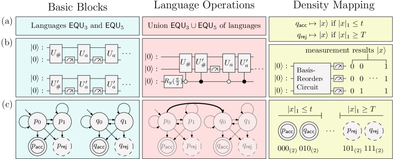
We propose a framework that addresses these challenges and enhances simulation accuracy by providing intuitive QFA composition methods alongside improvements to the transpilation process from QFAs to quantum circuits. Our framework enables users to compose complex QFAs from simple QFAs using language operations. Our proposed methodology extends the notable frameworks of classical automata, such as FAdo [17], FSA [18] and others [19, 20, 21, 22, 23, 24]. In our proposed framework, we also introduce the novel concept of density mapping, a method employed in our framework for determining the bit-representation of each state in a QFA during transpilation. Density mapping is designed to reduce the probability of fluctuation caused by bit-flip errors. Fig. 1 demonstrates how a user can compose and simulate quantum circuits using the proposed framework. The intended workflow of our proposed framework is threefold: (1) constructing simple QFAs, (2) combining these simple QFAs with language operations to compose a complex QFA and (3) transpiling the resulting complex QFA into a circuit using density mapping. The given workflow lends to a more intuitive approach to quantum circuit construction as well as improved simulation accuracy therein.
In summary, we propose a framework that facilitates the construction and accurate simulation of QFAs. Our main contributions are as follows.
-
1.
We introduce a novel QFA construction of unary finite languages, which serves as the elementary units of our framework.
-
2.
We prove closure properties of various language classes defined by QFAs to illustrate how our framework combines QFAs.
-
3.
We propose the -mapping technique to enhance the QFA simulation accuracy on quantum computers.
The rest of the paper is organized as follows. Section 2 provides a brief background on QFAs and their languages. In Section 3, we present details of our framework. We demonstrate the effectiveness of our density mapping in Section 4 by running experiments on the proposed framework. Finally, we summarize the results and outline possible future work in Section 5. Our framework is publicly accessible at https://github.com/sybaik1/qfa-toolkit.
2 Preliminaries
We first describe notations and definitions of two types of QFA: one is a measure-once (MO-) QFA and the other is a measure-many (MM-) QFA. We then define several types of languages recognized by MO-QFAs and MM-QFAs.
2.1 Basic Notations
Symbols and denote the set of real numbers and the set of complex numbers, respectively. For a finite set with elements, and denote the set of column vectors of dimensions and the set of matrices of sizes whose components are indexed by elements of and , respectively. For an element , is a unit vector whose components are all zero, except an -indexed component. The set is a standard basis of the vector space . A vector has a unique expression as a linear combination:
Then, denotes the length of .
We use , and to denote a transpose, inverse, conjugate and conjugate-transpose of a matrix , respectively. denotes the determinant of a given matrix . A matrix is considered unitary if it satisfies the equality: . Given a finite set of indices and a set , a projection matrix onto is a zero-one diagonal matrix where if and , otherwise. For matrices and with , their direct sum is
A superposition of qubits is formalized as a -dimensional complex vector with a length of 1, and its evolution is described by a unitary matrix. The basis vectors of the superposition are represented by , where each digit corresponds to the value of each qubit. The measurement of the superposition is formalized by an observable, which is a partitioning of the dimensions. When a superposition is measured with an observable, it collapses to one of the vectors , each with a probability .
2.2 Quantum Finite-State Automata and Languages
A finite-state automaton (FA) is a model that simulates the behavior of a system changing its state between a fixed number of distinct states. The automaton updates its state in an online manner in response to external inputs—formalized as strings over a finite alphabet. A quantum finite-state automaton (QFA) is a quantum variant of FA, which can exist in a superposition comprised of a finite number of states. We consider two different types of QFAs: an MO-QFA, which is observed only at the end of sequential inputs [25], and an MM-QFA, which is observed after every step of the sequence [11].
Let denote a finite input alphabet, which consists of the symbols used in sequential input. A semi-QFA then describes the evolution of a QFA for each symbol. Fig. 2 shows how transitions of a semi-QFA are represented graphically.
Definition 1.
A semi-QFA is a tuple , where (1) is a finite set of state, (2) is the unitary matrix for each symbol and (3) is the tape alphabet, with and as the start-of-string and end-of-string symbols, respectively.

We can define MO-QFAs and MM-QFAs as semi-QFAs with two defining distinctions: the inclusion of an initial state as well as that of final states, which are either accepting or rejecting.
Definition 2.
An MO-QFA is specified by a tuple111In some other papers, the tape alphabet of an MO-QFA does not include the end-of-string symbol. This does not affect the expressive power or the size of MO-QFAs [12]. , where (1) a triple is a semi-QFA; (2) is an initial state; and (3) is a set of accepting states.
An MO-QFA reads each symbol of string one by one and updates its superposition of states at each based on their transition matrix corresponding to the symbol. After reading the entire string, the MO-QFA measure the the superposition of states. It accepts the string if and only if the measured state is an accepting state; otherwise, it reject the string.
Formally, for a string on the tape alphabet, we denote the unitary matrix as . We also denote , and as , and , respectively, for simplicity of notation. Then, the probability of an MO-QFA accepting string is , where is the superposition of the QFA after reading the end-of-string symbol.
Definition 3.
An MM-QFA is specified by a tuple , where (1) is a semi-QFA; (2) is an initial state; (3) are sets of accepting and rejecting states, respectively. We denote a set of non-halting states
The MM-QFA reads the tape symbols one by one for a given string and updates the superposition according to the transition matrix, similar to MO-QFAs. However, unlike MO-QFAs, it measures their superposition at the end of each step, causing it to collapse onto one of three sub-spaces , or . The MM-QFA then accept or reject the string immediately if the resulting superposition is on the MM-QFA or , respectively. Otherwise, it keeps reading the next symbol.
Kondacs and Watrous [11] introduced total states to formalize the decision process of MM-QFAs. A total state is a triple , where and are the accumulated probabilities of acceptance and rejection. The vector denotes the superposition and the probability of non-halting by its direction and the square of its length, respectively. For an MM-QFA , is an evolution function of the internal state of with respect to defined as follows:
where
For a string on the tape alphabet, we use to denote . Then, denotes the final total state, and is the probability that accepts a given string .
We say that an MM-QFA is valid if for any . If for every such that , then we say that is end-decisive. In other words, does not accept strings before reading the end-of-string symbol. Similarly, is co-end-decisive if it only rejects strings when reading the end-of-string symbol [12]. For the rest of the paper, we focus solely on valid MM-QFAs.
Let be an MO-QFA or an MM-QFA and denote the probability that a given accepts . We call the function the stochastic language of . We say an MO- or MM-QFA recognizes with a positive one-sided error of margin if (1) for and (2) . In other words, always rejects and accepts with probability . Similarly, we say recognizes with a negative one-sided error of margin if (1) for and (2) for .
We define the following classes of quantum finite-state languages (QFLs) , , and as those recognized by MO-QFAs, MM-QFAs, end-decisive MM-QFAs and co-end-decisive MM-QFAs, respectively. We also define the class of complements for each language family, which are denoted using a prefix -. For example, denotes the class .
2.3 Closure Properties of Stochastic Languages of QFAs
Stochastic languages of QFAs possess known closure properties, specific to MO-QFAs under the following operations [25, 13, 26].
-
(Hadamard product)
-
(Convex linear combination)
For with ,
-
(Complement)
-
(Inverse homomorphism)
Compared to the stochastic languages of MO-QFAs, those of MM-QFAs are closed under linear combination, complement and inverse homomorphism [13, 27] but not under the Hadamard product. For the cases of end-decisive and co-end-decisive MM-QFAs, their stochastic languages are closed under linear combination and inverse homomorphism. However, end-decisive MM-QFAs, in particular, are also closed under the Hadamard product [27]. Table 1 summarizes the closure properties of stochastic languages of QFAs. We also present a construction for the convex linear combination to complete the paper.
| QFA Class | ||||
|---|---|---|---|---|
| MO-QFA | ✓ | ✓ | ✓ | ✓ |
| MM-QFA | ✗ | ✓ | ✓ | ✓ |
| End-dec. | ✓ | ✓ | ✓ | |
| Co-end-dec. | ✓ | ✓ |
Proposition 1.
Consider two MM-QFAs
-
1.
and
-
2.
For with , the following MM-QFA satisfies .
where for and
If and are both end-decisive or co-end-decisive, then the resulting is also end-decisive or co-end-decisive, respectively.
3 Proposed Framework for QFLs
It is more complex to construct QFAs as opposed to classic FAs due to the unitary constraints that a QFA must preserve. On top of the difficulties with QFAs, when constructing a quantum circuit that recognizes a QFL, one has to consider a margin with the accepting probability and rejecting probability—the accepting policy [12, 28]. Several accepting policies exist, such as one-sided errors, two-sided errors, isolated cut-points, threshold acceptance and threshold with margin [13]. In our framework, we only consider one-sided errors since they offer a compromise between the language coverage and the closure properties.
When designing a quantum circuit for a language, a typical process of making their QFA proceeds as follows: First, determine the number of states for the target QFA. Then, construct transition matrices for each of the states adhering to unitary constraints. Subsequently, verify if the created QFA can differentiate between accepting and rejecting strings. If it fails to do so, adjustments to the transitions design or an increase in the number of states are necessary. If the target QFA functions as intended, it can be transpiled into a quantum circuit.
The aforementioned process is not the sole paradigm of designing a circuit, but the continuous evolution of which, boasting both advancements and errors, are necessary in the development of the target quantum circuit. We overcome these errors and inconveniences by encapsulating the design process through the use of QFLs as building blocks. By doing so, we can employ operations between the building blocks to construct the desired QFL. In our framework, we provide constructions for the two languages and as building blocks, leveraging them to create more complex and diverse languages. In the above scenario, instead of deciding on the size and transitions, we can decompose the language into a set of expressions with and , then compose them to get the QFA. We can finally transpile the QFA with our density mapping to get the target quantum circuit.
3.1 Basic Blocks—Two QFLs with Simple Constructions
We settled on small and simple QFAs as the building blocks of our framework and give the characteristics and properties of two QFAs and .
First, we revisit that has several previous approaches due to its small and simple circuit [16]. It is known that there exists a two-state MO-QFA that recognizes the language with a negative one-sided bounded error. Furthermore, for each prime , there exists an -state MO-QFA recognizing with an error margin of , which is independent of the choice of . The circuit of and requires only one and qubits, respectively [28]. Next, we present our construction of an MM-QFA for .
Theorem 1.
Let be a unary alphabet. For a singleton language , and parameters with , let be an co-end-decisive MM-QFA defined as follows.
where The specific unitary operators are given by
where is a sub-matrix given by
and the factor is given by Then, recognizes the language with a negative error bound with a margin satisfying
Proof.
Fix for some parameters , and . The validity of is obvious from the construction. For each , let Then, the values of components are and . By induction, Now we consider the final total state The rejecting probability of a string is
and From the observation that we finally obtain
∎
One might need to execute the QFA matching process multiple times to obtain a correct result, as the probability of obtaining the correct results decreases with the increasing length of the input string. The subsequent theorem describes how many repetitions are required to achieve a predetermined probability of accuracy.
Theorem 2.
Fix the parameters and define and . Let for each . Then, for each , where
Proof.
Note that has the minimum reject probability when , except in the case where . We can compute the value of as follows:
Then, for . Therefore, when and are fixed independently of , one have to run on for -times to decide within a fixed probability. ∎
Note that Theorems 1 and 2 examine the condition where parameters and are chosen independently to the target language . The following proposition describes how our framework finds optimal parameters that maximize the error margin for each .
Proposition 2.
Let be a unique positive solution of . Then, parameters and maximize the error margin of .
Proof.
We want to maximize the rejection probability of where
Let be an objective function. Then, the following holds.
Since is differentiable on the domain , the equation holds. Then, we obtain the following equations from the partial derivatives of with respect to and .
| (1) | ||||
| (2) |
Then, from Eq.s (1) and (2), we derive
| (3) |
and
respectively. Combining these equations, we obtain
Therefore, if is a unique positive solution of an equation , then the optimal parameters are ∎
3.2 Closure Properties of QFLs
In our framework, we consider Boolean operation over , and distinguish the closure and error-bound properties of each operation. The closure operations are considered for each language class: , , and . These also include the basic constructions of each language. Unlike other classes that are defined based on cut-points as mentioned in previous literature[12, 28], the properties of these classes have only been indirectly discussed. We examine properties of one-sided error-bounded languages, including closure properties for operations, to clarify how our framework supports the operations.
From an MO- and MM-QFA, we can obtain their complement QFAs by exchanging the set of accepting states and the set of rejecting states. We establish the following properties from the construction that transforms an end-decisive MM-QFA from a co-end-decisive MM-QFA and vice versa.
Property 1.
and are the class of languages recognized by MO-QFAs and MM-QFAs with a bounded positive one-sided error, respectively.
The proof of Property 1 follows from the closure property of stochastic languages of QFAs under complement.
Proof.
Let be a . By definition, is a , meaning there exists an MO-QFA and a margin such that and . Given that stochastic languages are closed under complement, we can construct another MO-QFA such that . Therefore, and . Thus, MO-QFA recognizes with a bounded positive one-sided error. The proofs for the inverse direction are omitted for brevity. The proof for is straightforward and follows similarly. ∎
Property 2.
and are the class of languages recognized by co-end-decisive and end-decisive MM-QFAs with a bounded positive one-sided error, respectively.
Proof.
We show that the operations are closed under stochastic language and correlate with the properties of QFLs.
Theorem 3.
Each class , , and of languages is closed under intersection.
Proof.
The closure property of each language under intersection follows from the closure property of their corresponding QFAs under linear combination. ∎
Theorem 4.
and are closed under union.
Proof.
Let and be languages in . By Property 1, there exist MO-QFAs and recognizing and with a positive one-sided bounded error. Hence, there exists an MO-QFA satisfying due to the closure property of MO-QFAs under Hadamard product. recognizes with a positive one-sided error, and by Property 1 again, is a language. For the closure property of , we can utilize Property 2 instead of Property 1, and the closure property of end-decisive MM-QFAs with regard to the Hadamard product. ∎
The next statement directly follows the fact that there exists a co-end-decisive MM-QFA for each unary finite language. The corollary leverages the closure property of with regard to its union and the concept of singleton language construction from Theorem 1.
Corollary 1.
Every unary finite language is in .
Table 2 summarizes the upper bounds of operational complexities as well as the complexities of inverse homomorphism and word quotient—both of which can be easily established from the their constructions [25, 12].
| QFL Class | Union | Intersection | Inverse Homo. () | Word Quotient () |
| and denote the and , respectively. | ||||
3.3 Density Mapping from QFA States to Qubit Basis Vectors
After a user composes QFAs for their QFLs using either simple constructions or language operations, the next step is to transpile these QFAs into quantum circuits. In the implementation of a QFA in a quantum computer with qubits, each state of the QFA is represented with -bits as one of basis vectors and the transitions are realized through a combination of quantum gates. Additionally, in the current era of noisy intermediate-scale quantum computing [29], we need to apply error mitigation methods that can compensate for possible errors.

We propose a technique called density (-) mapping which is applied before the transpilation stage of the quantum circuit. Rather than mapping QFA states to qubit basis vectors in an arbitrary manner, our -mapping reorders these vectors based on the number of qubits with value . Then we assign the accepting and rejecting states to the basis vectors with a low and high number of qubits having the value , respectively.
-mapping maximizes the localization of accepting and rejecting states, thereby reducing the probability of bit-flip errors. These errors can arise from a decoherence or depolarization, and causes an accepting state to change into a rejecting state, and vice versa. Additionally, the basis vectors representing the accepting and rejecting states are separated by basis mapped to non-final states and basis that are not mapped to any states. This method helps to isolate the errors and reduce possible error situations. Fig. 3 conceptually illustrates how our proposal reduces a bit-flip error from altering the acceptance of a QFA.
4 Experimental Results and Analysis
We demonstrate the effectiveness of our -mapping with experiments using our framework. Our experiments measure how accurately quantum circuits simulate an operation of of states and of states by default construction. We compare the difference between ideal and experimental acceptance probabilities with and without the -mapping. We take 100,000 shots and measure the number of acceptances and rejections for each string.
We use IBM’s Falcon r5.11 quantum processor for real quantum experiments. When simulating the quantum circuits with controlled error rates, we utilize Qiskit simulators222https://www.ibm.com/quantum/qiskit. The Qiskit simulator is configured to use the same basis gates and topological structure as the Falcon processor. We also set the error rates to follow the Falcon processor, except for the two types of errors—gate and readout errors. A mirroring factor is applied to each error rate of gate in the processor. The error rate of in the simulator is calculated as follows:
Readout errors are adjusted using the mirroring factor and the readout error in the simulator is calculated similarly.
4.1 Difficulty of QFA simulation
We measured the language using the Falcon processor, as depicted in Fig. 4. This measurement was to demonstrate the current capabilities and state of quantum computers. Note that the automaton of accepts strings of length divisible by with probability . Otherwise, it accepts the string with a probability less than 0.875. However, we can see that the measurements for the real-world computer accept strings with a probability close to 0.5. We analyze the low accuracy attributed to the large size of the resulting quantum circuit, exceeding 1,000 gates for even a length 2 input.
We also notice despite the small error rates of the simulator, the output of the simulator becomes inaccurate as the length of the string becomes longer. The inaccuracy is caused by the size of the circuit that grows linearly to the length of the input string. The accumulated errors eventually dominate and reduce the output closer to random guessing.
Our experiments from this point on are conducted using a quantum simulator to focus on the effectiveness of -mapping. We use error mirroring rates designed to reflect the capabilities of near-future quantum computers with error suppression and mitigation.

4.2 Effectiveness of the Density Mapping on Simulators
We demonstrate the usefulness of our -mapping for emulating QFAs. We evaluate the accepting probability of input strings with the automaton of implemented by quantum circuits. Fig. 5 compares the experimental results for two quantum circuits recognizing , one utilizes our mapping and the other does not.

The experimental results confirm that -mapping increases the accuracy of the simulation for most cases. The mapping increases the accepting probability of strings in up to length and decreases the accepting probability of strings that are not in . The effectiveness of -mapping diminishes with longer strings. Both mapping methods are increasingly affected by accumulating errors as discussed in Section 4.1, resulting in similar outcomes.
4.3 Effectiveness of the Density Mapping in Various QFAs
Table 3 presents the mean absolute percentage error (MAPE) of the experimental results for and implementations using the naive mapping and -mapping. Each cell denotes the dissimilarity between ideal probabilities and measured for inputs , and a simulation with a lower MAPE indicates higher accuracy. MAPE is calculated as follows:
We use strings with length from to to compute the MAPE for each language. Note that the maximum achievable value of MAPE varies for each language, hence we cannot directly compare simulation accuracy between different languages using MAPE. For instance, consider the following cases: (1) and ; and (2) and , where the latter case has greater error rate. Nevertheless, we use the according formulation to shows the difference between probabilities and its difference.
| M.F. (%) | Naive Mapping | Density Mapping | |||||||||||||
| 5 | 7 | 5 | 7 | 3 | 5 | 7 | 3 | 5 | 7 | ||||||
| 0.1 | 2.49 | 1.64 | 1.35 | 0.07 | 0.08 | 0.07 | 1.43 | 1.32 | 1.35 | 0.06 | 0.07 | 0.07 | |||
| 0.1 | 0.5 | 2.90 | 1.35 | 1.25 | 0.09 | 0.09 | 0.10 | 1.44 | 1.17 | 1.65 | 0.09 | 0.10 | 0.09 | ||
| 1 | 2.82 | 1.85 | 1.43 | 0.10 | 0.11 | 0.08 | 1.92 | 1.21 | 1.66 | 0.13 | 0.11 | 0.10 | |||
| 0.1 | 12.76 | 7.44 | 5.80 | 0.10 | 0.09 | 0.11 | 6.13 | 4.85 | 6.22 | 0.11 | 0.11 | 0.11 | |||
| 0.5 | 0.5 | 13.08 | 7.16 | 6.01 | 0.14 | 0.17 | 0.13 | 6.24 | 4.64 | 6.04 | 0.14 | 0.13 | 0.16 | ||
| 1 | 12.86 | 7.10 | 5.87 | 0.19 | 0.17 | 0.20 | 6.08 | 4.85 | 6.25 | 0.18 | 0.15 | 0.18 | |||
| 0.1 | 24.18 | 13.83 | 11.02 | 0.19 | 0.21 | 0.18 | 11.66 | 8.39 | 10.94 | 0.19 | 0.19 | 0.19 | |||
| 1 | 0.5 | 24.26 | 13.73 | 10.91 | 0.23 | 0.20 | 0.23 | 11.37 | 8.28 | 11.21 | 0.22 | 0.18 | 0.22 | ||
| 1 | 24.46 | 13.94 | 11.18 | 0.25 | 0.23 | 0.29 | 11.31 | 8.36 | 11.15 | 0.24 | 0.26 | 0.27 | |||
The experimental results indicate that -mapping is effective for QFAs of languages , , but not for . -mapping reduces the difference between the accepting probabilities of ideal results and simulation for to of the former case and of the latter case. Similarly, for , -mapping reduces the difference to and of the former and latter case, respectively.
Note that the number of quantum circuit for increases with the growth of . We observe that the effect of -mapping is not evident for , as the simulation remains inaccurate regardless of the mapping used. This emphasizes the challenge posed by the large size of QFAs and the resulting quantum circuits, which involve a significant number of gates.
We also examine the impact of -mapping on QFAs of , although its effect is less pronounced compared to . Note that QFAs of are MM-QFAs. Unlike MO-QFAs for , simulations of MM-QFAs have the possibility of terminating before reading all symbols in each string. We suggest that the simulation for MM-QFAs receives less effect from gate errors because they may ignore trailing gates, thereby resulting in the reduced effectiveness of -mapping.
The overall experimental results reveal that gate error rates dominate simulation accuracy for QFAs, and our experiments do not show a clear relation between readout error rates and simulation accuracy. This is primarily due to the fact that the quantum circuits for QFAs have few measurement gates.
5 Conclusions and Future Work
MO-QFA and MM-QFA are the two most simplest quantum computational models. Despite their simple structure, designing these models is complex because their transitions must satisfy the unitary constraints. Verification is also challenging due to the low accuracy of current quantum devices. We have developed the framework to facilitate easy construction and accurate simulation of QFAs. For the development of the framework, we have
-
•
composed a novel construction for ,
-
•
demonstrated the closure properties of , , and ,
-
•
introduced -mapping to improve the accuracy of experiments on real-world devices,
-
•
showcased the basic functionalities of our framework.
Our experiments on real devices highlight a significant limitation of current quantum processors—the QFA simulations on these processors are close to the random guessing due to their low accuracy. On the other hand, the experimental results confirm that our density mapping increases the accuracy of the QFA simulations.
A major limitation of our framework is its inability to construct QFAs from a human-readable format while most FA frameworks support a direct FA construction from regular expressions. Furthermore, manual construction remains inevitable for some languages because some types of QFLs cannot be obtained by composing and . We aim to characterize the class of languages by identifying which languages and operations can generate these classes. We will then integrate these languages and operations into our framework and enable users to construct a broader variety of languages more easily.
Our density mapping technique reduces simulation errors by correlating each QFA state with an appropriate dimension of a quantum circuit. The accuracy in quantum circuits can also be increased by reducing the number of gates [16] or by assigning more physical qubits to represent a single logical qubit [30]. The interaction between the density mapping and these existing methods may affect their overall effectiveness. Thus, it is another future work to integrate our density mapping with other techniques for improving the overall performance.
References
- Benioff [1980] Paul Benioff. The computer as a physical system: A microscopic quantum mechanical hamiltonian model of computers as represented by Turing machines. Journal of statistical physics, 22:563–591, 1980. doi: https://doi.org/10.1007/BF01011339.
- Emu et al. [2023] Mahzabeen Emu, Salimur Choudhury, and Kai Salomaa. Quantum neural networks driven stochastic resource optimization for metaverse data marketplace. In 2023 IEEE 9th International Conference on Network Softwarization (NetSoft), pages 242–246, 2023. doi: https://doi.org/10.1109/NetSoft57336.2023.10175433.
- Arrazola et al. [2020] Juan Miguel Arrazola, Alain Delgado, Bhaskar Roy Bardhan, and Seth Lloyd. Quantum-inspired algorithms in practice. Quantum, 4:307, 2020. doi: 10.22331/q-2020-08-13-307.
- Hagan and Wiebe [2023] Matthew Hagan and Nathan Wiebe. Composite quantum simulations. Quantum, 7:1181, 2023. doi: 10.22331/q-2023-11-14-1181.
- King [2023] Robbie King. An improved approximation algorithm for quantum max-cut on triangle-free graphs. Quantum, 7:1180, 2023. doi: 10.22331/q-2023-11-09-1180.
- Nishimura and Ozawa [2009] Harumichi Nishimura and Masanao Ozawa. Perfect computational equivalence between quantum Turing machines and finitely generated uniform quantum circuit families. Quantum Information Processing, 8:13–24, 2009. doi: https://doi.org/10.22331/q-2023-03-20-956.
- Nishimura [2003] Harumichi Nishimura. Quantum computation with restricted amplitudes. International Journal of Foundations of Computer Science, 14(05):853–870, 2003. doi: https://doi.org/10.1142/S0129054103002059.
- Gainutdinova and Yakaryılmaz [2018] Aida Gainutdinova and Abuzer Yakaryılmaz. Unary probabilistic and quantum automata on promise problems. Quantum Information Processing, 17:1–17, 2018. doi: https://doi.org/10.1007/s11128-017-1799-0.
- Vieira and Budroni [2022] Lucas B Vieira and Costantino Budroni. Temporal correlations in the simplest measurement sequences. Quantum, 6:623, 2022. doi: https://doi.org/10.22331/q-2022-01-18-623.
- Huang et al. [2023] Ruo Cheng Huang, Paul M Riechers, Mile Gu, and Varun Narasimhachar. Engines for predictive work extraction from memoryful quantum stochastic processes. Quantum, 7:1203, 2023. doi: https://doi.org/10.22331/q-2023-12-11-1203.
- Kondacs and Watrous [1997] Attila Kondacs and John Watrous. On the power of quantum finite state automata. In 38th Annual Symposium on Foundations of Computer Science, FOCS ’97, Miami Beach, Florida, USA, October 19-22, 1997, pages 66–75, 1997. doi: https://doi.org/10.1109/SFCS.1997.646094.
- Brodsky and Pippenger [2002] Alex Brodsky and Nicholas Pippenger. Characterizations of 1-way quantum finite automata. SIAM Journal on Computing, 31(5):1456–1478, 2002. doi: https://doi.org/10.1137/S0097539799353443.
- Bertoni et al. [2003] Alberto Bertoni, Carlo Mereghetti, and Beatrice Palano. Quantum computing: 1-way quantum automata. In Developments in Language Theory, 7th International Conference, DLT 2003, Szeged, Hungary, July 7-11, 2003, Proceedings, volume 2710, pages 1–20, 2003. doi: https://doi.org/10.1007/3-540-45007-6_1.
- Ambainis et al. [1999] Andris Ambainis, Ashwin Nayak, Ammon Ta-Shma, and Umesh Vazirani. Dense quantum coding and a lower bound for 1-way quantum automata. In Proceedings of the thirty-first annual ACM symposium on Theory of computing, pages 376–383, 1999. doi: https://doi.org/10.1145/301250.301347.
- Giannakis et al. [2015] Konstantinos Giannakis, Christos Papalitsas, and Theodore Andronikos. Quantum automata for infinite periodic words. In 2015 6th International Conference on information, intelligence, systems and applications (IISA), pages 1–6. IEEE, 2015. doi: https://doi.org/10.1109/IISA.2015.7388105.
- Birkan et al. [2021] Utku Birkan, Özlem Salehi, Viktor Olejár, Cem Nurlu, and Abuzer Yakaryilmaz. Implementing quantum finite automata algorithms on noisy devices. In Computational Science - ICCS 2021 - 21st International Conference, Krakow, Poland, June 16-18, 2021, Proceedings, Part VI, volume 12747, pages 3–16, 2021. doi: https://doi.org/10.1007/978-3-030-77980-1_1.
- Almeida et al. [2009] André Almeida, Marco Almeida, José Alves, Nelma Moreira, and Rogério Reis. FAdo and GUItar. In Implementation and Application of Automata, 14th International Conference, CIAA 2009, Sydney, Australia, July 14-17, 2009. Proceedings, volume 5642, pages 65–74, 2009. doi: https://doi.org/10.1007/978-3-642-02979-0_10.
- Kanthak and Ney [2004] Stephan Kanthak and Hermann Ney. FSA: An efficient and flexible C++ toolkit for finite state automata using on-demand computation. In Proceedings of the 42nd Annual Meeting of the Association for Computational Linguistics (ACL-04), pages 510–517, 2004. doi: https://doi.org/10.3115/1218955.1219020.
- Mousavi [2016] Hamoon Mousavi. Automatic theorem proving in Walnut. arXiv, abs/1603.06017, 2016. doi: https://doi.org/10.48550/arXiv.1603.06017.
- Mohri et al. [1997] Mehryar Mohri, Fernando C. N. Pereira, and Michael Riley. A rational design for a weighted finite-state transducer library. In Automata Implementation, Second International Workshop on Implementing Automata, WIA ’97, London, Ontario, Canada, September 18-20, 1997, Revised Papers, volume 1436 of Lecture Notes in Computer Science, pages 144–158. Springer, 1997. doi: https://doi.org/10.1007/BFb0031388.
- Allauzen et al. [2007] Cyril Allauzen, Michael Riley, Johan Schalkwyk, Wojciech Skut, and Mehryar Mohri. OpenFst: A general and efficient weighted finite-state transducer library. In Jan Holub and Jan Zdárek, editors, Implementation and Application of Automata, 12th International Conference, CIAA 2007, Prague, Czech Republic, July 16-18, 2007, Revised Selected Papers, volume 4783, pages 11–23, 2007. doi: https://doi.org/10.1007/978-3-540-76336-9_3.
- May and Knight [2006] Jonathan May and Kevin Knight. Tiburon: A weighted tree automata toolkit. In Implementation and Application of Automata, 11th International Conference, CIAA 2006, Taipei, Taiwan, August 21-23, 2006, Proceedings, volume 4094, pages 102–113, 2006. doi: https://doi.org/10.1007/978-3-031-07469-1.
- Arrivault et al. [2017] Denis Arrivault, Dominique Benielli, François Denis, and Rémi Eyraud. Scikit-SpLearn: a toolbox for the spectral learning of weighted automata compatible with scikit-learn. In Conference francophone sur l’Apprentissage Aurtomatique, 2017. URL https://hal.science/hal-01777169/.
- Brainerd [1969] Walter S. Brainerd. Tree generating regular systems. Information and Control, 14(2):217–231, 1969. doi: https://doi.org/10.1016/s0019-9958(69)90065-5.
- Moore and Crutchfield [2000] Cristopher Moore and James P. Crutchfield. Quantum automata and quantum grammars. Theoretical Computer Science, 237(1-2):275–306, 2000. doi: https://doi.org/10.1016/S0304-3975(98)00191-1.
- Ambainis et al. [2001] Andris Ambainis, Arnolds Ķikusts, and Māris Valdats. On the class of languages recognizable by 1-way quantum finite automata. In Annual Symposium on Theoretical Aspects of Computer Science, pages 75–86, 2001. doi: https://doi.org/10.1007/3-540-44693-1_7.
- Bianchi and Palano [2010] Maria Paola Bianchi and Beatrice Palano. Behaviours of unary quantum automata. Fundamenta Informaticae, 104(1-2):1–15, 2010. doi: https://doi.org/10.3233/FI-2010-333.
- Ambainis and Freivalds [1998] Andris Ambainis and Rusins Freivalds. 1-way quantum finite automata: Strengths, weaknesses and generalizations. In 39th Annual Symposium on Foundations of Computer Science, FOCS ’98, November 8-11, 1998, Palo Alto, California, USA, pages 332–341, 1998. doi: https://doi.org/10.1109/SFCS.1998.743469.
- Preskill [2018] John Preskill. Quantum computing in the NISQ era and beyond. Quantum, 2:79, 2018. doi: https://doi.org/10.22331/q-2018-08-06-79.
- Ghosh et al. [2012] Joydip Ghosh, Austin G Fowler, and Michael R Geller. Surface code with decoherence: An analysis of three superconducting architectures. Physical Review A, 86(6):062318, 2012. doi: https://doi.org/10.1103/PhysRevA.86.062318.