∎
Department of Applied Mathematics
King Abdullah University of Science and Technology, Saudi Arabia22institutetext: 22email: [email protected] 33institutetext: Department of Mathematics, Raiganj University, West Bengal, India
33email: [email protected]
44institutetext: Department of Mathematics and Statistics , IIT Kanpur, Uttar Pradesh, India
44email: [email protected] 55institutetext: Department of Mathematics, Raganj University, India
A Fractional Image Inpainting Model Using a Variant of Mumford-Shah Model
Abstract
In this paper, we propose a fourth order PDE model for image inpainting based on a variant of the famous Mumford-Shah (MS) image segmentation model. Convexity splitting is used to discrtised the time and we replace the Laplacian by its fractional counterpart in the time discretised scheme. Fourier spectral method is used for space discretization. Consistency, stability and convergence of the time discretised model has been carried out. The model is tested on some standard test images and compared them with the result of some models existed in the literature.
Keywords:
Image Processing Inpainting Fourth Order Partial differential equation (PDE)Convexity splitting.1 Introduction
Image inpainting is a process of filling in the missing part of an image from the information available outside the missing part. In mathematical term it is an extrapolation of the image. Although there are several inpainting methods are available in the literature, we consider the Partial differential equation (PDE) based methods because of its sound established theory.
Since image inpainting is relatively new topic in the field of image processing, a lot of inpainting models are based on the models of denoising and segmentation. Like in CS1 Chan and Shen have used a modified version of Rudin-Osher-Fatemi (ROF) denoising model rof for image inpainting and the resulting inpainting model is known as inpainting model. Following the model a series of models sch ; CS2 ; CS3 have been proposed which fall in the category of variational inpainting. In variational inpainting, the PDE is obtained by minimizing an energy functional of the following form:
| (1) |
where is the given damaged image and is the inpainted image and
| (2) |
with and is the damaged part of the image. The term is called regularization term, is called fidelity term and is called fidelity parameter which forces the inpainting image to remain closer to the original image outside the missing/ degraded region .
Another variational model for inpainting has been proposed by Esedoglu and Shen mse . They have brought the Mumford-Shah model of segmentation and used it for image inpainting. The Mumford-Shah(MS) functional is non-convex and contains an unknown set of lower dimension, so it is difficult to solve the minimization problem. Several approximations have been proposed in the literature surveyMS . Esedoglu and Shen mse have used the Ambrosio and Tortorelli’s approximation of the MS energy functional for the inpainting model. Applying the gradient descent to the approximations give raise to a parabolic problem of second order with a parameter . Since the second order models are not good for inpainting tvh , as second order models are unable to fill large gaps, they have modified their second order model using Euler-Elastica energy to get a fourth order model in the same paper mse , known as Mumford-Shah-Euler (MSE) model.
The parameter of the MSE model reminds the authors of mCH about the Cahn-Hilliard equation used to model phase-separation phenomena of material science. They have modified the Cahn-Hilliard equation and proposed a model for image inpainting in mCH . Here after we will call this model as mCH model. The mCH model has few drawbacks, like it is applicable for binary images only. Then several authors have come up with inapinting models cCH ; fCH ; anis ; lininp ; nonlininp by modifying the Cahn-Hilliard model to overcome the drawbacks of mCH model.
More recently, Cai et.al. twophase have proposed a segmentation model which is also derived from the Mumford-Shah model. This segmentation model is also used for inpainting in the subsequent paper of the same authors in threephase . But this model will leads to second order equation. As we know that the second order model are not able to fill large gaps tvh , so we will propose a fourth order model in this article using a variant of the MS functional. We will use convexity splitting tvh in time and Fourier spectral methods in space for the proposed model.
The paper is organised is as follows: In section 2 we have discussed some relevant existing models and thereby proposed our model. Section 3, talks about convexity splitting and the numerical scheme for our proposed model. Also we have established the consistency, stability and convergence of the time discretised model. Further, we have introduced the fractional time discretised model. In section 4, we have presented the fractional version of the time discretized scheme and present the scheme with complete discretization. Then the numerical results of our model have been presented and compared them with the same of models like and and the second order model of Cai et.al. twophase . Finally, in section 5 we draw some conclusions.
2 Proposed model and some existing models
In this section, we will discuss few inpainting models from the literature which are relevant to us and then proposed our model.
2.1 and model
The inpainting model and are of variational type that is they are obtained by minimizing an energy functionl of the form (1). For both the models the regularization term is the total variation of that is . The fidelity term for the model is and is .
With the above choices, the minimizing energy of the model is :
| (3) |
The gradient descent of the corresponding Euler-Lagrange equation is
| (4) |
To avoid division by zero the above equation is modified CS1 as:
| (5) |
where is a parameter.
Similarly, we get the PDE for the model as
| (6) |
2.2 Mumford-Shah model
As we have mentioned in the introduction that our model will be derived from MS-model. In MS- model on has to minimize the following energy functional
| (7) |
where are parameters and is a curve inside the image domain But the functional is non-convex, so it is not solvable directly. So there are several simplified version has been proposed like proposed in twophase ; mse . A detail survey on Mumford-Shah model and its variant applied to image processing can be found in surveyMS .
In twophase authors have proved that minimizing the functional (7) is equivallent to minimizing the following functional:
| (8) |
For segmentation is constant throughout the domain but for inpainting is some constant outside the damaged part and zero in . Changing the fidelity parameter of the model (8), the same model has been used in threephase in context of colour image which is of the form:
| (9) |
where is defined in (2). The corresponding Euler-Lagrange equation will be
| (10) |
which is equivalent to solve the steady state solution of the equation
| (11) |
Here after we will call this model as convex variant of Mumford-Shah (CVMS) model.
2.3 Proposed Model
But this is a second order model so it will not be able to fill large gap. So we will propose a higher order model. To do this we modify the MS-functional as follows:
| (12) |
then following the steps of twophase we can prove that this is equivalent to minimising
| (13) |
Now using the regularized version of the total-variation the functional reduced to:
| (14) |
where is a small parameter. For all numerical results presented in this work we choose . The corresponding descent model will be
| (15) |
| Image |
|
|
|
|
|
|
||||||
|---|---|---|---|---|---|---|---|---|---|---|---|---|
| Dog | 1 | 37.50 | 30.46 | 0.9412 | 2999 | 17.29 | ||||||
| 1.2 | 38.78 | 31.73 | 0.9704 | 1580 | 9.13 | |||||||
| 1.4 | 39.14 | 32.09 | 0.9767 | 950 | 5.41 | |||||||
| 1.6 | 39.13 | 32.09 | 0.9764 | 830 | 4.80 | |||||||
| 1.8 | 39.02 | 31.97 | 0.9758 | 810 | 4.74 | |||||||
| 2 | 38.88 | 31.83 | 0.9748 | 720 | 4.21 | |||||||
| GrayShade | 1 | 35.11 | 31.41 | 0.7853 | 1180 | 9.10 | ||||||
| 1.2 | 42.39 | 38.69 | 0.9627 | 1200 | 9.37 | |||||||
| 1.4 | 44.73 | 41.03 | 0.9872 | 1210 | 9.16 | |||||||
| 1.6 | 45.39 | 41.69 | 0.9925 | 1220 | 9.10 | |||||||
| 1.8 | 45.40 | 41.70 | 0.9925 | 1170 | 9.15 | |||||||
| 2 | 45.38 | 41.67 | 0.9925 | 1200 | 9.42 |
| Image |
|
|
|
|
|
|
|
|||||||
|---|---|---|---|---|---|---|---|---|---|---|---|---|---|---|
| GrayShade | 41.64 | 37.94 | 0.9822 | 33965 | =10 | 18.81 | ||||||||
| 45.23 | 41.54 | 0.9909 | 6576 | =10 | 38.84 | |||||||||
| Our | 45.40 | 41.70 | 0.9925 | 1210 | =1.8 | 8.90 | ||||||||
| Kaleidoscope | 26.24 | 18.51 | 0.8827 | 66365 | =50 | 52.35 | ||||||||
| 26.90 | 19.17 | 0.8770 | 2280 | =50 | 22.87 | |||||||||
| Our | 27.89 | 20.16 | 0.9130 | 2020 | =1.8 | 23.07 | ||||||||
| Elephant 1 | 35.02 | 28.20 | 0.9694 | 2720 | =200 | 12.47 | ||||||||
| 33.93 | 27.12 | 0.9396 | 2030 | =200 | 11.41 | |||||||||
| Our | 36.16 | 29.35 | 0.9694 | 490 | =1.4 | 3.96 | ||||||||
| Elephant 2 | 27.53 | 20.71 | 0.9009 | 2400 | =500 | 10.64 | ||||||||
| 28.29 | 21.47 | 0.8997 | 756 | =500 | 4.78 | |||||||||
| Our | 28.51 | 21.70 | 0.8961 | 260 | =1.8 | 2.27 | ||||||||
| Dog | 38.68 | 31.63 | 0.9867 | 40265 | =500 | 14.37 | ||||||||
| 38.13 | 31.09 | 0.9758 | 3946 | =500 | 18.01 | |||||||||
| Our | 39.14 | 32.09 | 0.9764 | 830 | =1.6 | 4.80 |
| Image |
|
|
|
|
|
|
|
|||||||
|---|---|---|---|---|---|---|---|---|---|---|---|---|---|---|
| Lena 1 | 31.58 | 25.92 | 0.9167 | 1091 | =100 | 14.45 | ||||||||
| CVMS | 31.99 | 26.33 | 0.9174 | 645 | =100 | 8.63 | ||||||||
| Our | 32.92 | 27.27 | 0.9321 | 450 | =1.6 | 9.57 | ||||||||
| Lena2 | 34.86 | 29.20 | 0.9456 | 1990 | =100 | 26.91 | ||||||||
| CVMS | 34.97 | 29.31 | 0.9451 | 835 | = 100 | 11.30 | ||||||||
| Our | 35.62 | 29.96 | 0.9597 | 945 | =1.4 | 19.55 | ||||||||
| Lena3 | 26.08 | 20.42 | 0.7972 | 11550 | =10 | 159.31 | ||||||||
| CVMS | 27.67 | 22.01 | 0.8808 | 1520 | =100 | 21.32 | ||||||||
| Our | 28.34 | 22.68 | 0.8963 | 1795 | =1.4 | 37.60 | ||||||||
| Barbara 1 | 26.93 | 21.04 | 0.8851 | 1265 | =100 | 16.74 | ||||||||
| CVMS | 27.70 | 21.81 | 0.8867 | 970 | =100 | 13.10 | ||||||||
| Our | 28.33 | 22.45 | 0.9055 | 485 | = 1.2 | 10.40 | ||||||||
| Barbara 2 | 29.87 | 23.98 | 0.9346 | 1890 | =100 | 25.72 | ||||||||
| CVMS | 30.56 | 24.67 | 0.9340 | 1020 | =100 | 13.74 | ||||||||
| OUR | 31.40 | 25.52 | 0.9505 | 1055 | =1.2 | 22.09 | ||||||||
| Barbara3 | 23.10 | 17.21 | 0.6797 | 7660 | =10 | 105.13 | ||||||||
| CVMS | 25.77 | 19.88 | 0.8547 | 1330 | =100 | 17.96 | ||||||||
| OUR | 26.42 | 20.53 | 0.8720 | 1610 | =1.2 | 35.52 |
3 Convexity splitting and numerical scheme
We will solve our proposed model (15) using the convexity splitting in time and Fourier spectral method in space. We replaced the Laplacian in the time discretized scheme by its fraction version and get the fractional time discretized model of the proposed model. Convexity splitting methods are used to solve gradient system. Split the energy functional into a convex part and a concave part and in the time discretized scheme the convex part is considered implicitly and the other one explicitly.
The proposed model (15) can be obtained as the gradient flow of the energies and in norm where
| (16) |
To apply convexity splitting idea we split as and as where
and
where are positive and should be large enough so that for becomes convex.
So the semi-discrete time-stepping scheme for our model is
| (17) |
Simplifying we get the time discretized model as:
| (18) |
with the boundary condition
| (19) |


Now, we replace the Laplacian in (3) by it’s fractional counterpart in the spirit of fCH and obtained a fractional model. In general, fractional models are more effective and flexible for image processing problems fCH . So the equation (3) reduces to:
| (20) |
with the boundary condition
| (21) |
Here is fractional power for We know that the Laplacian has a complete orthonormal eigenvectors satisfying the Neumann boundary condition corresponding to eigenvalues . Consider the eigenvalue problem in
for where
Let us define the space fCH ,
| (22) |
Then for any , the fractional Laplace operator can be defined by
| (23) |
Hence has the same interpretation as in terms of its spectral decomposition. Fourier spectral methods represent the truncated series expansion when a finite number of orthonormal eigenfunction is considered. Consistency, stabilit and convergence of the time discretized model for the case has been carried out in the Appendix B and the analysis for the fractional one is a matter of future research as it need fractional Green’s type theorem to prove the results. Taking Fourier transform of (3) and using the spectral decomposition of Laplacian (23) we get
| (24) |
where . In every time step we will calculate the and the real part of the inverse Fourier transform will be the solution .
4 Numerical results and discussion
In this section, we present some numerical results on few standard test images and compared them with the results of and model. For our model, we set the parameters as and , the fidelity parameter and the constant occurred in convexity splitting is set as The fractional parameter is different for different images which is mentioned in the corresponding table. For comparison we have used the code of and provided in codeinp . To compare the quality of the results we calculate three quality metrics namely peak signal to noise ratio (PSNR), siganl to noise ratio (SNR) and structural similarity index measure (SSIM) ssim . PSNR is the ratio between the maximum possible value of the original image and the mean squared error between the original and the resulting image in log scale and SNR is the ratio between the variance of the original image and the variance of the noise. SSIM represents the geometric similarity of the resulting image with the original image. For all the three quality metrics, higher the value implies better the result.
To investigate the performance with different fractional power , we have tested our model with different values of on few images. In Fig. 1, we have shown the inpainting results of dog image withe different value of namely . The results corresponding to are not good enough. We have calculated the quality metrics PSNR, SNR, and SSIM for all the results and reported them in Table 1. From the table one can see that for and the results are better than the others specially better than the results of the cases when is an integer. Thus the model with fractional power is better than the the usual model.
Similarly, we have tested our model on grayshade image for different values of . The inpainted results are shown in Fig. 2. To compare the results we have calculated PSNR, SNR and SSIM for all the cases and reported in Table 1. From the table one can see that in this case gives the best result in this case.
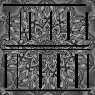
Now we will compare results of our model with that of and model. In Fig. 3, we have taken two images namely Grayshade image and Kaleidoscope image and corresponding damaged image has been shown in the first row. Inpainted results of all the three models for the grayshade image are presented in second row and results of Kaleidoscope image in third row. From the figure one can see that the results of is not good and results of and our model is better. For both the images the fractional power is chosen as 1.8. PSNR, SNR and SSIM for these images are reported in Table 2. From the table one can see that for Grayshade image our model gives little better result. For the Kaleidoscope image our model gives much better result than the results of the other two model. For example, SSIM for model is 0.87 whereas SSIM for our model is 0.91.
In Fig. 4, we have presented the results of two images namely Elephant and dog. We have taken two different damaged region for the elephant image and one damage region for the dog image and all the damaged images are shown in the first row of Fig. 4. Inpainted results are shown in row two, three and four. The first column contains results of model, second column contains the result of and results of our model is displayed in third column. For these image the fractional parameter of our model is chosen as 1.4,1.8 and 1.6 respectively. From the table one can see that for all the case our model perform better than other two models in terms of PSNR, SNR and SSIM. For the Dog and first elephant image there is significant improvement in the performance in our model.
In the next two experiments, we have compared our results with the results obtained by and CVMS twophase model. For the CVMS model we have discretized the equation (11) by convexity splitting in time and Fourier spectral method in space which is presented in Appendix A.
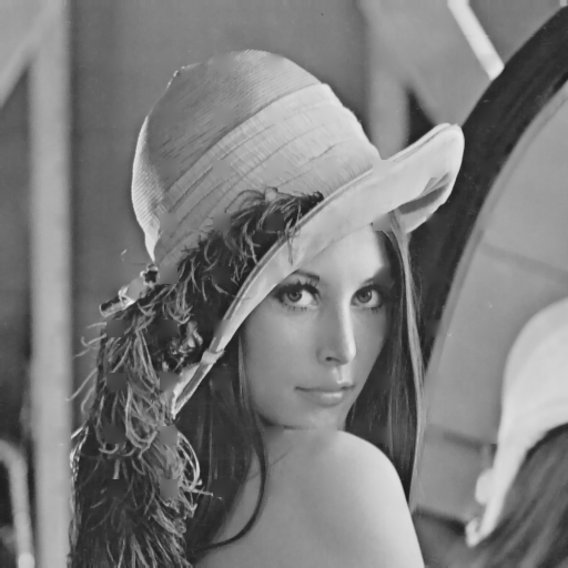
First experiment is on Lena image of size . We select three different inpainting domain for Lena image and the corresponding damaged images are shown in the first row of Fig. 5. The results of first damaged image have been shown in second row and the results of second damaged image have been shown in third row and results of third damaged image is shown in fourth row. From the fourth row of Fig. 5 one can see that our model is giving better result than the other two. For all the models we have reported image quality metrics PSNR, SNR, and SSIM in Table 3. Also the best fractional power is mentioned for each image in the same table. From the Table 3, it is evident that our model perform better than the other two models in terms of PSNR, SNR, and SSIM.
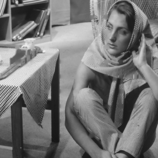
Finally, we did the experiment on the Barbara image of size . Three different inpainting domain are chosen and the resulting degraded images are shown in the first row of Fig. 6. The results of model have been shown in first column, second column contains the result of CVMS model twophase and our results are in third column. In this case, also we can observe from the Table 3 our model perform much better than the other two in terms of PSNR, SNR and SSIM. Note that the Barbara image contains some structures and preserving them is a challenge and in this case also our model gives better result.
5 Conclusion
Here we have presented a new 4th order PDE model for grayscale image inpainting using a variant of Mumford-Shah model. Convexity splitting in time has been used for time discretization and further the time discretized model has been modified by replacing the Laplace term by its fractional version. Fourier spectral method in space has been to get the complete discretization. Consistency, stability and convergence have been established for the time discretized scheme. Numerical results show the superiority of our model over and and convex variant of Mumford-Shah model.
Appendix A
The equation (11) can be written as gradient descent of two functional in where
| (25) |
To apply convexity splitting idea we split as and as where
and
where are positive and should be large enough so that for becomes convex.
So the semi-discrete time-stepping scheme for our model is
| (26) |
Simplifying we get the time discretized model as:
| (27) |
To get the complete discretized scheme we will use Fourier spectral method in space. Let be the discrete Fourier trans form of . Taking Fourier transform of (Appendix A) and using the relation and rearranging we get the final numerical scheme for the first model as:
| (28) |
where and is matrix with size with
Appendix B
Now, we will discuss the consistency, stability and convergence of the time discretized model (3) that is for the fractional model with
Theorem 5.1 (Consistency, Stability and Convergence)
Let be the exact solution of (15) and be the exact solution at time for a time step and Let be the -th iterate of(3) with constant . Then the following statements are true:
-
(a)
Under the assumption that and are bounded, the numerical scheme is consistent with the continuous equation and of order one in time.
-
(b)
the solution is bounded on a finite time interval , for all . In particular for , fixed, we have for every
(29) -
(c)
The discretization error . For smooth solution and , the error converges to as . In particular we have for , fixed, that
for suitable constants
Proof
Proof
(b) Consider the time discretized scheme
| (31) |
Multiplying the time discretised scheme (Proof) by and integrating over we get
Using Young’s inequality on the product terms we get,
| (32) |
Using the following two estimates nondenoising in (Proof)
| (33) |
and
| (34) |
we get,
Let us choose and , we get,
Since , all the coefficients are positive. Now multiplying both sides by we get,
| (35) |
where . Dividing both sides by we get,
| (36) |
Choose in such a way that and (this is possible if we choose big enough ), then above equation reduces to
| (37) |
So by induction we will get,
| (38) |
Expressing as = and using the inequality , we get for ,
| (39) |
References
- (1) M. Burger, L. He and C. Schonlieb, Cahn-Hilliard inpainting and a generalization for grayvalue images, SIAM J. Imaging Sci., 2 (4), 1129-1167, 2009.
- (2) C.B. Schonlieb, and A. Bertozzi, Unconditionally stable schemes for higher order inpainting.Commun. Math. Sci. 9 (2) (2011) 413-457.
- (3) X. Cai, R. Chan, and T. Zeng, A Two-Stage Image Segmentation Method Using a Convex Variant of the Mumford–Shah Model and Thresholding, SIAM Journal of Imaging Sciences, vol. 6(1), pp. 368-390, 2013.
- (4) X. Cai, R. Chan, M. Nikolova, and T. Zeng, A Three-Stage Approach for Segmenting Degraded Color Images: Smoothing, Lifting and Thresholding (SLaT). J Sci Comput 72, 1313–1332 (2017).
- (5) T.F. Chan and J. Shen, Mathematical models for local non-texture inpaintings, SIAM J. Appl. Math., 62(3), 1019-1043, 2001.
- (6) T.F. Chan and J. Shen, Non-texture inpainting by curvature driven diffusions (CDD), J. Visual Commun. Image Rep., 12(4), 436-449, 2001.
- (7) T.F. Chan, S.H. Kang and J. Shen, Euler’s elastica and curvature-based inpainting, SIAM J. Appl. Math., 63(2), 564–592, 2002.
- (8) L. I. Rudin, S. Osher and E. Fatemi, Nonlinear total variation based noise removal algorithms, Physica D, 60, 259-268, 1992.
- (9) S. Esedoglu and J.H. Shen, Digital inpainting based on the Mumford-Shah-Euler image model, Eur. J. Appl. Math., 13(4), 353-370, 2002.
- (10) L. Bar, T. F. Chan, G. Chung, M. Jung, N. Kiryati, N. Sochen, and L. A. Vese, Mumford and Shah Model and its Applications to Image Segmentation and Image Restoration. In: Handbook of Mathematical Methods in Imaging. Springer, New York, NY, 2011.
- (11) A. Bertozzi, S. Esedoglu and A. Gillette, Inpainting of binary images using the Cahn-Hilliard equation, IEEE Trans. Image Proc., 16(1), 285-291, 2007.
- (12) A. Bertozzi, S. Esedoglu and A. Gillette, Analysis of a two-scale Cahn-Hilliard model for image inpainting, Multiscale Modeling and Simulation, 6(3), 913-936, 2007.
- (13) T.F. Chan, J.H. Shen and H.M. Zhou, Total variation wavelet inpainting, J. Math. Imaging Vis., 25(1), 107-125, 2006.
- (14) L. Cherfils, H. Fakih and A. Miranville, A complex version of the Cahn-Hilliard equation for grayscale image inpainting, Multiscale Model. Simul. 15 (2017), 575-605.
- (15) J. Bosch and M. Stoll, A Fractional Inpainting Model Based on the Vector-Valued Cahn-Hilliard Equation, SIAM Journal on Imaging Sciences, vol. 8(4), pp. 2352-2382, 2015.
- (16) Anis Theljani, Zakaria Belhachmi, Moez Kallel, Maher Moakher. Multiscale Fourth- Order Model for Image Inpainting and Low-Dimensional Sets Recovery. 2016.
- (17) B.V.R. Kumar, A. Halim, A Linear Fourth Order PDE Based Grayscale Image Inpainting Model, Computational and Applied Mathematics, vol. 38(1), pp. 1-21,2019.
- (18) A. Halim, B.V.R. Kumar, An anisotropic PDE model for image inpainting, Computers and Mathematics with Applications, vol.79(9), pp. 2701–2721, 2020.
- (19) Z. Wang, A.C. Bovik, H.R. Sheikh, and E.P. Simoncelli, Image quality assessment: from error visibility to structural similarity, IEEE Transactions on Image Processing, vol. 13 (4), pp. 600–612, 2004.
- (20) A. Halim, B.V. R. Kumar, A PDE model for effective denoising, Computers and Mathematics with Applications, vol. 80(9) , pp. 2176–2193, 2020.
- (21) C.B. Schnlieb, Higher-order total variation inpainting - File Exchange - MATLAB Central.