A Flow-Based Generative Model for Rare-Event Simulation

First let us introduce a mathematical basis for rare-event simulation and Importance Sampling. Consider a random object (e.g., random variable, random vector, or stochastic process), $\boldsymbol{X}$, taking values in some space, $\mathcal{X}$, with probability density function, $p(\boldsymbol{x})$, that represents the result of a simulation experiment. Running simulations corresponds to sampling $\boldsymbol{X}$. We consider rare events of the form $\{\boldsymbol{X}\in\mathcal{A}\}$, where $\mathcal{A}\subset\mathcal{X}$ is the set of simulation outcomes $\boldsymbol{x}$ that satisfy a predicate ${S(\boldsymbol{x})\geq\gamma}$ for some performance function $S:\mathcal{X}\rightarrow\mathbb{R}$ and level parameter $\gamma\in\mathbb{R}$. The probability $c$ of the rare event $\{\boldsymbol{X}\in\mathcal{A}\}$ can thus be written as

where $c$ is very small, but not 0. Here, $\mathbbm{1}_{\mathcal{A}}(\boldsymbol{x})$ is an indicator function that is 1 when ${\boldsymbol{x}\in\mathcal{A}}$ and 0 otherwise, and $\mathbb{E}$ represents the expected value. The expected number of simulations to sample a single rare event is $1/c$, so simulating rare events by sampling $\boldsymbol{X}$ directly quickly becomes computationally infeasible the rarer the event is. Therefore, other techniques, such as Importance Sampling become necessary to simulate and analyse rare events.

In particular, suppose that $\boldsymbol{X}$ is sampled from a probability density function $p(\boldsymbol{x})$ and that we wish to estimate the quantity

via “crude” Monte Carlo: Simulate $\boldsymbol{X}_{1},\ldots,\boldsymbol{X}_{n}$ independently from $p$, and estimate $\ell$ via the sample average $\sum_{i=1}^{n}H(\boldsymbol{X}_{i})/n$. The idea of Importance Sampling is to change the probability distribution under which the simulation takes place. However, computing the expected value of a function of $\boldsymbol{X}$ while using a different sampling density $q$, requires a correction factor of the likelihood ratio $p(\boldsymbol{x})/q(\boldsymbol{x})$,

where ${\mathbb{E}}_{p}={\mathbb{E}}$ and ${\mathbb{E}}_{q}$ represent the expected values under the two probability models. This relationship allows an unbiased estimate of $\ell$ to be computed by sampling $\boldsymbol{X}$ from $q$ instead of $p$, via

where $\boldsymbol{X}_{1},\ldots,\boldsymbol{X}_{n}$ is an independent and identically distributed (iid) sample from $q$. Note that any choice for $q$ is allowed, as long as $q(\boldsymbol{x})\neq 0$ when $p(\boldsymbol{x})\neq 0$. The optimal sampling distribution for estimating $\ell$ in this way is thus the distribution that minimizes the variance of the estimator $\widehat{\ell}$. When $H$ is strictly positive (or strictly negative), choosing the probability density

yields in fact a zero-variance estimator, because then $\widehat{\ell}=\ell$. As a special case, an unbiased estimator of the rare-event probability $c={\mathbb{P}}(\boldsymbol{X}\in A)$ can be computed as

and the optimal sampling density $q^{*}$ is just the original density $p$ truncated to the rare-event region $\mathcal{A}$:

More generally, if we want to estimate the expectation of $H(\boldsymbol{X})$ conditional on $\boldsymbol{X}\in\mathcal{A}$, that is,

then $\ell^{\mathcal{A}}$ can be estimated via

In this case, the optimal Importance Sampling density is

If it is possible to approximate the target density (e.g., the optimal Importance Sampling density) closely, then we are able to compute certain quantities of interest (e.g., $c={\mathbb{P}}(\boldsymbol{X}\in\mathcal{A})$ or $\ell={\mathbb{E}}H(\boldsymbol{X}))$ with low variance. Normalizing Flows is a generative model that can closely approximate a wide variety of probability densities. Suppose the random object, $\boldsymbol{X}$, can be mapped to another random object, $\boldsymbol{Z}$, taking values in some space $\mathcal{Z}$ of the same dimensionality, and vice versa, via invertible differentiable functions $\boldsymbol{\psi}$ and $\boldsymbol{\phi}=\boldsymbol{\psi}^{-1}$, so that

where $\boldsymbol{u}$ is a vector representing all, if any, parameters. If, under the target density, $\boldsymbol{\phi}$ maps $\boldsymbol{X}$ to a random object $\boldsymbol{Z}$ that has a simple base distribution, such as a (multivariate) normal or uniform distribution, then the target distribution can be sampled indirectly by sampling from the base distribution and mapping the result using $\boldsymbol{\psi}$. The name of such a generative model is derived from the idea that a sequence of invertible differentiable transformations can map even a very complex probability distribution to a simple base distribution, thereby forming a ‘normalizing flow’. The construction of the ‘flow’ relies on the principle that any composition of invertible differentiable functions will also be invertible and differentiable.

In what follows, we assume that $\cal X$ is a subset of $\mathbb{R}^{n}$ and that $\boldsymbol{X}$ and $\boldsymbol{Z}$ are “continuous” random variables; more precisely, that they have probability densities $p_{\boldsymbol{X}}$ and $p_{\boldsymbol{Y}}$ with respect to the Lebesgue measure on $\cal X$. Since $\boldsymbol{\psi}$ is differentiable, the probability density function $\boldsymbol{X}$ can be expressed in terms of the probability density function $\boldsymbol{Z}$ via the relation

or, in terms of $\boldsymbol{z}$:

Here, $\mathrm{D}\boldsymbol{\phi}(\boldsymbol{x}\mathchar 24635\relax\;\boldsymbol{u})$ is Jacobian matrix of $\boldsymbol{\phi}$ and the absolute value of its determinant is the Jacobian of $\boldsymbol{\phi}$, and similar for $\boldsymbol{\psi}$. If $\boldsymbol{\psi}$ is a composition of other invertible differentiable functions,

then we can use the chain rule to combine the Jacobians as a product,

Therefore, analogous to a feed-forward neural network, the full Jacobian can be computed during a single pass as $\boldsymbol{\psi}(\boldsymbol{z}\mathchar 24635\relax\;\boldsymbol{u})$ is computed. A similar result holds for the inverse: $\boldsymbol{\phi}$. Functional composition increases the complexity of the model while maintaining the accessibility of the Jacobian. In this way, Normalizing Flows provides the opportunity for highly expressible generative models, with computationally tractable density functions. As will be discussed in Section 2.4, training the model to learn a target density from a given function, rather than via training data, requires the ability to compute $p_{\boldsymbol{X}}$ as a differentiable function. Therefore, using a Normalizing Flows model improves and simplifies the framework introduced by Gibson \BBA Kroese (\APACyear2022) by eliminating the need to train a second neural network to approximate the density function via kernel density estimation.

Coupling Flows, first introduced by Dinh \BOthers. (\APACyear2015), is a family of Normalizing Flows which have been shown to be universal approximators of arbitrary invertible differentiable functions when composed appropriately (Teshima \BOthers., \APACyear2020). A single Coupling Flows unit splits $\boldsymbol{z}$ into two vectors, $\boldsymbol{z}^{A}$ and $\boldsymbol{z}^{B}$, as well as $\boldsymbol{x}$ into $\boldsymbol{x}^{A}$ and $\boldsymbol{x}^{B}$. It then transforms one part via an invertible differentiable function, $\boldsymbol{w}$, called the coupling function, which contains parameters determined by the other partition. The relationship between the second part and the coupling function parameters, called the conditioner, $\Theta$, does not need to be invertible, since this part is not transformed and is accessible when computing the inverse. This means functions with many learnable parameters, like neural networks, can be used to capture interesting and complex dependencies between variables. Figure 1 illustrates the structure of a Coupling Flow models and its inverse.

The Coupling Flow can be expressed mathematically as:

Note that the parameters $\boldsymbol{u}$ of the flow are contained in the conditioner, $\Theta$. Since the $B$-partition does not transform, the Jacobian of the full transformation is just the Jacobian of the coupling function; that is,

The coupling function is often chosen to be a simple affine transformation (Dinh \BOthers., \APACyear2015, \APACyear2016; Kingma \BBA Dhariwal, \APACyear2018). Instead, we base our coupling function on the rational function proposed by Ziegler \BBA Rush (\APACyear2019):

This function has five parameters when applied elementwise. However, separate parameters can be used for each dimension in the $\boldsymbol{z}^{A}$ partition. For additional complexity, the coupling function can also be a composition of these rational functions, $w(\cdot\mathchar 24635\relax\;\Theta)=\operatorname*{\circ}_{i}r_{i}(\cdot\mathchar 24635\relax\;\theta_{1}^{i},\theta_{2}^{i},\theta_{3}^{i},\theta_{4}^{i},\theta_{5}^{i})$. In this case the total number of parameters in the coupling function is five multiplied by the number of compositions multiplied by the number of dimension in $\boldsymbol{z}^{A}$. We choose the conditioner function to be a Multilayer Perceptron, with an input dimensionality to match $\boldsymbol{z}^{B}$ and an output dimensionality to match the number of parameters in the coupling function.

In order for eq. 10 to define an invertible function, some restrictions have to be placed on the parameters. Choosing

ensures that the function $r$ in eq. 10 is a strictly increasing invertible function. We enforce these constraints, following Ziegler and Rush, by processing the output of the conditioner Multilayer Perceptron,

where primed letters denote unconstrained outputs of the conditioner function. The factor of 0.95 in the expression for $\theta_{3}$ helps improve stability by precluding barely invertible functions that can exist near the bound $|\theta_{3}|=8\sqrt{3}\theta_{1}/(9\theta_{4})$. While we do not need to compute the inverse in our method, it can be calculated as the real solution to a cubic equation.

A single coupling flow unit does not transform the $B$-partition. So, functional composition is necessary to obtain a general approximation. To achieve this, the dimensions of each coupling flow unit are split differently to ensure that all dimensions have to opportunity to ‘influence’ all other dimensions, thereby capturing any dependencies between all dimensions. In practice, we permute the dimensions between Coupling Flow units, while fixing the partitioned dimensions. The permutation of dimensions can be viewed as special case of a linear transformation, where the transformation matrix is a permutation of the rows of the identity matrix. The Jacobian matrix of a linear transformation is equal to the transformation matrix. So, the Jacobian is just 1 and is trivial to include in the probability density calculations of eq. 8 and eq. 9.

Choosing an appropriate Normalizing Flows model architecture allows any density to be approximated arbitrarily well if the correct parameters can be identified. We use a form of stochastic gradient descent to iteratively tune the parameters of the model to minimize the Kullback–Leibler (KL) divergence between the model density, $q$ say, and a known target function, $h:\mathcal{X}\rightarrow\mathbb{R}$, that is proportional to the target probability density function. That is, we minimize

Note that a model density $q$ that minimizes eq. 11 also minimizes the KL divergence between $q$ and the actual (normalized) target density. The advantage of using eq. 11 is that the normalization constant of the target density does not need to be known. This motivates the following minimization program:¹¹1Actually, the first term in this objective corresponds to the negative differential entropy of the base density and does not depend on any parameters, so could be omitted. However, we keep it to make interpreting the loss a little simpler.

which corresponds to choosing parameters to minimize the KL divergence between the Normalizing Flows generative density and a target density whose probability density function is proportional to $h$. The expression can be derived by substituting $q$ from eq. 9 into eq. 11 and taking the expectation with respect to the base density. The minimum KL divergence is zero, when the two densities are identical, so the minimum value of this objective is the negative natural logarithm of the normalization constant of $h$. For example, if $h(\boldsymbol{x})=p(\boldsymbol{x})H(\boldsymbol{x})$, then the minimum value of the objective function $L$ is $-\ln\ell$. The objective function values can be estimated via

where $\boldsymbol{Z}_{1},\ldots,\boldsymbol{Z}_{n}$ is an iid sample of the base density.

The objective function $L$ marks a clear distinction between how we train a Normalizing Flows generative model using a target function, and how they are typically trained using a data set. In other works, such as by Dinh \BOthers. (\APACyear2015), Normalizing Flows are trained to learn the density of a data set by maximizing the log-likelihood of the sampled data. While this can be considered equivalent to minimizing the KL divergence, the training process involves sampling the data set, which corresponds to sampling $\boldsymbol{X}$, and then moving in the ‘normalizing’ direction with $\boldsymbol{\phi}$ to solve the maximization program:

After the model is trained, new data can be generated by sampling $\boldsymbol{Z}$ and moving in the ‘generating’ direction using $\boldsymbol{X}=\boldsymbol{\psi}(\boldsymbol{Z}\mathchar 24635\relax\;\boldsymbol{u})$. Therefore, in the data-focused case, it is essential to be able to compute both transformations, $\boldsymbol{\psi}$ and $\boldsymbol{\phi}$. However, in the context of rare-event simulation, we do not have access to training data, but a target function that is proportional to a target probability density, and all training occurs in the ‘generating’ direction. Therefore, computing $\boldsymbol{\phi}$ is not required (although $\boldsymbol{\psi}$ must still be invertible in principle). Algorithm 1 outlines our training procedure.

As previously shown in eq. 4 and eq. 7, when estimating rare-event probabilities and other quantity conditioned on a rare event, the target density includes an indicator function, $\mathbbm{1}_{\mathcal{A}}(\boldsymbol{x})$. However, the term, $-\ln h(\boldsymbol{\psi}(\boldsymbol{Z}\mathchar 24635\relax\;\boldsymbol{u}))$ in the objective function $L$ in eq. 12 requires each value $h(\boldsymbol{x})$ of the target function value to be strictly positive. To circumvent this problem, we reuse the solution presented by Gibson \BBA Kroese (\APACyear2022), to approximate $\mathbbm{1}_{\mathcal{A}}(\boldsymbol{x})$ by defining a strictly positive penalty factor,

which is a positive approximation of $\mathbbm{1}_{\mathcal{A}}(\boldsymbol{x})$ when $\alpha>0$ and $\mathcal{A}^{c}=\{\boldsymbol{x}\in\mathcal{X}~{}|~{}S(\boldsymbol{x})<\gamma\}$ is the complement set of $\mathcal{A}$. The approximation is more accurate the larger the value of $\alpha$ and is exact in the limit $\alpha\rightarrow\infty$. Figure 2 illustrates the convergence of the approximation.

Therefore, if the target density includes the indicator function as a factor, we replace it with the penalty factor with appropriate performance function, $S$. For example, if the aim is to estimate $\ell^{\mathcal{A}}$ from eq. 5, then the target function would be of the form

Note that in this case

so learning a conditional density by including the penalty factor in the target function is equivalent to learning the unconditional target $p(\boldsymbol{x})H(\boldsymbol{x})$ and including an additional penalty term in the objective that penalizes samples outside the rare-event region. In this way, $\alpha$ can be interpreted as the weight of the penalty. For our experiments we choose $\alpha=100$.

Firstly we consider a very simple one-dimensional example of a truncated normal density. Let $X$ have a standard normal distribution: $X\sim\mathcal{N}(0,1)$ and consider the rare-event region $\mathcal{A}=[\gamma,\infty)$. An obvious choice for the performance function is $S(x)=x$, so if the goal is to estimate the rare-event probability $c={\mathbb{P}}(X\geq\gamma)$, then the target function is

A Coupling Flow is unsuitable for a one-dimensional problem, so we use a composition of three rational functions from eq. 10, containing a total of 15 parameters. Choosing a batch size of $n=1,000$, a learning rate of $0.001$, a weight decay parameter of $0.0001$ and $\alpha=100$, the model was trained via Algorithm 1 and the Adam gradient descent optimizer (Kingma \BBA Ba, \APACyear2017) for 30,000 iterations. Figure 3 illustrates how the model converges towards the truncated normal target density, with threshold parameter $\gamma=3$.

Using a sample of 1,000 points, eq. 3 gives us an estimate 0.00134576 of the rare-event probability ${\mathbb{P}}(X\geq 3)$ , which is about 0.3% error from the true value of about 0.0013499. From the same sample, the sample standard deviation is about 0.000261. We can estimate the minimum sample size needed for a 1% standard error by

where $\sigma$ is the sample standard deviation of the summand in eq. 3. Using a crude Monte Carlo estimator, the relative standard error should be $\sqrt{c(1-c)}\approx 0.0367$, requiring a much larger sample size of about $n=7.4\times 10^{6}$ for a 1% standard error.

The learned density is not exactly identical to the target conditional density, but is very close. To quantify how good the approximation is, we can estimate the KL divergence between the target density $q^{*}$ and the learned density using

In this example the KL divergence is estimated to be $0.03465$ with a standard error of $0.56\%$ using sample size 10,000.

Secondly, we try another example from Gibson \BBA Kroese (\APACyear2022) of a two-dimensional exponential density. In particular, in this example the probability density function of $\boldsymbol{X}=(X_{1},X_{2})$ is:

and the rare-event region is $\mathcal{A}=\{(x_{1},x_{2})\in\mathbb{R}^{2}_{+}~{}:~{}x_{1}+x_{2}\geq\gamma\}$, with performance function, $S(x_{1},x_{2})=x_{1}+x_{2}$. To estimate $c={\mathbb{P}}(X_{1}+X_{2}\geq\gamma)$, the target function is

This time we choose a flow model composed of six Coupling Flows, interlaced with dimension permutations, followed by an elementwise exponential function. The exponentiation ensures that the generated points are positive. The coupling function in each Coupling Flow is a composition of two rational functions of the form in eq. 10. The conditioner in each Coupling Flow is a linear transformation plus a constant vector. Therefore, the total number of learnable parameters is 60. Figure 4 shows the structure of this model via a flow chart.

The model was trained for 100,000 iterations with a learning rate of 0.0001, a weight decay of constant of 0.0001, and a batch size of 10,000. When $\gamma=10$, $c=(1+\gamma)\mathrm{e}^{-\gamma}\approx 0.000499399$. After training, with a sample size of 1,000 the estimated constant is $0.00049920$, with standard deviation of about $6.34\times 10^{-5}$ giving a relative standard error of 0.40%. Achieving a comparable standard error using a crude Mote Carlo estimator would require a sample size of more than $10^{8}$. Figure 5 shows how well the model learned the target density by including a scatter plot of a sample of points as well as comparing the learned probability density with the target probability density. The KL-divergence is estimated to be about 0.011 with 9.7% standard error using sample size of 10,000.

This third example comes from Chapter 9 of Kroese \BOthers. (\APACyear2011). In this example, we increase the number of dimensions to five, each corresponding to a random edge length in a bridge network, shown in Figure 6. The graph contains five edges and four nodes, where the length of each edge is uniformly distributed and the goal is to identify the expected shortest path from node $A$ to node $D$. Specifically, we wish to estimate the expected length of the shortest path from $A$ to $D$; that is, the expectation $\ell$ in eq. 1, with $X_{i}\sim\mathcal{U}(0,1)$ and

In this case $p(\boldsymbol{x})=1$, so the optimal Importance Sampling density that minimizes the variance in estimating $\ell$ is $q^{*}(\boldsymbol{x})=H(\boldsymbol{x})/\ell$. Therefore, the target function is $h(\boldsymbol{x})=H(\boldsymbol{x})$.

The space of allowed values in this example is $\mathcal{X}=[0,1]^{5}$, so it is reasonable to choose a model architecture in which the domains and co-domains of each composed flow unit is $[0,1]^{5}$. To achieve this we choose a uniform base distribution, $Z_{i}\sim\mathcal{U}(0,1)$. Additionally, the model is composed of five Coupling Flows and dimension permutation pairs. In each permutation the dimensions are cycled via $[3,4,5,1,2]$. The dimensions are partitioned so the coupling function transforms the first three dimensions. The coupling function of each Coupling Flow is a rational function based on eq. 10 with separate parameters for each dimension. The conditioner, like the previous example, is a linear transformation. Figure 7 uses a flow chart to illustrate the structure of this model. The parameters in the coupling functions of each Coupling Flow unit contain additional constraints to ensure that $r(0)=0$ and $r(1)=1$, thereby preserving the domain of $[0,1]^{5}$ at each flow component.

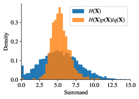
The model was trained with a learning rate of 0.0001, weight decay parameter of 0.0001, batch size 10,000 for 300,000 iterations. The scatter plot in Figure 8 compares the learned probability density of $\boldsymbol{\psi}(\boldsymbol{Z}\mathchar 24635\relax\;\boldsymbol{u})$ with the optimal sampling density given by eq. 2. The learned density forms a fairly good approximation of the optimal sampling density with a KL divergence of about 0.0017 with 29% standard error (using sample of 10,000). The histograms in Figure 8 compare the densities of the summands of the Importance Sampling estimator from eq. 1 and the crude Monte Carlo estimator, being the sample mean of $H(\boldsymbol{X})$. In this example both methods provide accurate estimates of the expected minimum path length. Typical values of the crude Monte Carlo and IS estimators are 0.9272 with a standard relative error of $0.43\%$ and 0.9301 with a standard relative error of $0.053\%$. While both values agree with the theoretical value of $l=\frac{1339}{1440}=0.92986\dot{1}$, the IS estimator reduces the variance by a factor of about 65.

In this example we continue with the bridge network, but now consider the rare event that the shortest path includes three edges, passing through the middle, rather than just two. That is, the shortest path is either $ABCD$ or $ACBD$. The rare-event region can be defined by choosing

and $\gamma=0$. That is, the penalty depends on the difference between the shortest ‘inner’ path ($ABCD$ or $ACBD$) and the shortest ‘outer’ path ($ABD$ or $ACD$).

The exact same model was reused, but trained across 500,000 iterations with the penalty factor included in the target function. In this way, the goal is to estimate the expected shortest path length of the distribution conditioned on the shortest path being $ABCD$ or $ACBD$. The rare event probability can be estimated using eq. 3 with a sample size of 10,000 to be about 0.0346 with a standard relative error of $1.3\%$. This corresponds to a variance reduction in a factor of about 17 compared to the crude Monte Carlo estimate. The conditional expected shortest path length can now be estimated via eq. 6 as 0.913 with a standard relative error of $1.7\%$.

By learning an approximation of the conditional distribution, we can explore the likely conditions required to generate the rare event. Figure 9 compares scatter plots between the learned unconditional and the conditional distributions. The unconditional distribution is not too different from the original uniform distribution, with the exception of $X_{1}$ and $X_{4}$. This is the expected result since the path, $ABD$, with path length $X_{1}+X_{4}$, is the most likely to be the shortest. However, the learned conditional distribution is significantly different to the original uniform distribution. From the scatter plots it is clear that $X_{3}$ is almost always short, and $X_{2}$ and $X_{5}$ have a strong negative correlation. Therefore, we can conclude that the most likely conditions for the shortest path to be one that passes through the middle edge, is that the middle edge is short, and that exactly one of bottom two edges is short. This is congruent with expectations since a long middle edge would likely make the total path length longer than both of the outer paths, if both bottom edges were short then the middle edge would be bypassed, and if both bottom edges were long, then the shortest path would likely be across the top.

In this section we look at stock price models and expected pricing of call options. This example, from Chapter 15 of Kroese \BOthers. (\APACyear2011), specifically looks at estimating the expected Asian call option of a stock whose undiscounted price, $S_{t}$, at time $t$ can be modelled by the Stochastic Differential Equation (SDE)

where the drift, $r$, is the risk-free rate of return, $\{X_{t}\}$ is a Wiener process and $\sigma$ is the volatility. This SDE is solved by

The average stock price across the interval $t\in[0,T]$ can be approximated by

where the time has been discretized into $n$ equal intervals of $\Delta t=T/n$,

and $X_{t_{i}}\sim\mathcal{N}(0,\Delta t)$. The discounted payoff at time $t=0$ of the Asian option is

where $\boldsymbol{X}=\left(X_{t_{1}},\ldots,X_{t_{n}}\right)$ and the $+$ superscript denotes the ramp function. Since $\{X_{t}\}$ is a Wiener process, $\boldsymbol{X}\sim\mathcal{N}(\mathbf{0},\Delta tI)$, where $I$ is the identity matrix of appropriate dimensionality. If the goal is to estimate the expected discounted payoff then, according to eq. 2, the optimal sampling distribution should include a factor of $H(\boldsymbol{x})$. However, the objective eq. 12 requires the target function to be non-zero at all sampled values. Therefore, we introduce the following approximation

which is a strictly positive continuously differentiable function that is exact in the limit $\delta\rightarrow 0$. In our experiments we choose $\delta=0.5$. Therefore, the target function is

We chose the base distribution to be $\boldsymbol{Z}\sim\mathcal{N}(\mathbf{0},\Delta tI)$ and the normalizing flow to be comprised of six coupling flow units with equal partition sizes. The dimensions were permuted after each coupling flow unit. Figure 10 illustrates the normalizing flows structure.

The parameters used in this example were $r=0.07$, $\sigma=0.2$, $K=35$, $S_{0}=40$, $T=4/12$ and $n=88$. The model was trained for 30000 steps with a batch size of 1000, learning rate of 0.0001 and weight decay of 0.0001. Figure 11 compares the histograms of the crude Monte Carlo and importance sampling estimator summands. Using a sample of 10000, the crude estimator is about 5.3432 with a standard relative error of $0.49\%$, and the importance sampling estimator is about 5.3580 with a standard relative error of $0.23\%$. This corresponds to a variance reduction of about a factor of 4.4.

Let us explore the rare event in which the discounted payoff exceeds 14, ${\mathcal{A}=\{\boldsymbol{x}\in\mathbb{R}^{n}~{}:~{}\mathrm{e}^{-rT}(\bar{S}_{T}-K)^{+}\geq\gamma\}}$ with performance function $S(\boldsymbol{x})=\mathrm{e}^{-rT}(\bar{S}_{T}-K)\geqslant\gamma$ and $\gamma=14$. In this case the goal is to explore how this rare event occurs and to estimate the probability of the rare event. Therefore, the target function is just the probability density function of the Wiener process multiplied by the penalty factor,

This time the model was trained for 100000 iterations. With a sample of 10000 the crude and IS estimators are about 0.0022 with $21\%$ relative error, and 0.0015797 with $0.46\%$ relative error respectively. This corresponds to a variance reduction of a factor of about 2100. Using the estimated normalization constant of 0.0015797 the KL divergence between the learnt density and the target density is about 0.15157 with a standard relative error of $0.40\%$ indicating that the learnt distribution is very close to the target conditional distribution. Figure 12 illustrates the strong linear relationship between the learnt log density and the target unconditional density, and compares the distributions of the simulated discounted Asian options.

Since the learnt distribution is a decent approximation of the conditional distribution, we can use the simulated trajectories to gain insights into how high performing options can occur. Figure 13 shows typical stock prices across time when simulating using the original probability measure and the learnt probability measure. In the first instance the average value is largely static, increasing very slowly, while the variance grows across time. However, conditioning the simulation on achieving a discounted payoff of at least 14 changes the trend unexpectedly. Rather than a steady growth in stock price across the whole time interval, most of the stock price growth occurs by $t=0.25$. Additionally, the variance is fairly constant over time during this growth time, mostly growing near the end. This result is also visible in the covariance matrix of the stock price, illustrated in figure 14. Under the original probability distribution the stock price near maturity depends little on the early prices, and the variance grows roughly linearly with time. However, under the learnt probability distribution, the variance in stock price is largely constant until a short time before maturity. Additionally, there is a small correlation between early stock prices and late stock prices. This could indicate that

In this example we test our method on a high-dimensional problem. A dimensionless particle traverses an unbounded $2$-dimensional environment for a maximum duration of $T$, which is discretized into $\Delta t=\frac{d}{2}$ time steps, where ${d\geq 2}$. The environment consists of a barrier with two slits, located at $(x_{\mathrm{slit}},y_{\mathrm{slit}})$ and $(x_{\mathrm{slit}},-y_{\mathrm{slit}})$. The width of both slits is $w_{\mathrm{slit}}$. Additionally, the environment contains a vertical screen located at $x_{\mathrm{screen}}$. The aim of the particle is to reach the screen while simultaneously passing through one of the two slits. At time step $0$, the particle starts at the $2D$-position $\boldsymbol{V}_{0}=(0,0)$. Given a random vector $\boldsymbol{Q}\sim\mathcal{N}(\boldsymbol{0},\frac{2T}{d}I_{d})$, where $I_{d}$ is the $d$-dimensional identity matrix, the position of the particle at time step $1\leq k\leq d/2$ evolves according to

where $\boldsymbol{Q}_{k}=(Q_{2k-1},Q_{2k})^{\top}$ is the $k$-th component vector of $\boldsymbol{Q}$. The path $\boldsymbol{V}$ of the particle induced by $\boldsymbol{Q}$ is then the sequence of points $\boldsymbol{V}=(\boldsymbol{V}_{k})_{k=1}^{d/2}$, with $\boldsymbol{V}_{k}$ defined according to eq. 15.

Let $g_{d}$ be the density of $\mathcal{N}(\boldsymbol{0},\frac{2T}{d}I_{d})$. Our goal is to learn a sampling density that is proportional to $g_{d}$ truncated to the rare-event region $\mathcal{A}=\left\{\boldsymbol{q}\in\mathbb{R}^{d}:S(\boldsymbol{q})\geq 0\right\}$, where $\boldsymbol{q}$ is an outcome of $\boldsymbol{Q}$. The performance function $S(\boldsymbol{q})$ is defined as follows. Suppose is $M$ is the time step where $\boldsymbol{X}$ is closest to the screen; that is,

where $X_{k}$ is the $x$-coordinate of the particle at time step $k$. Additionally, let $N$ be the first step where $X_{N-1}\leq x_{\mathrm{slit}}\leq X_{N}$, i.e., where the particle crosses $x_{\mathrm{slit}}$. The performance function of an outcome $\boldsymbol{q}$ of $\boldsymbol{Q}$, with path $\boldsymbol{v}=P(\boldsymbol{q})$, and outcomes $n$ and $m$ of $N$ and $M$ is then defined as

where

The functions $f_{1}$ and $f_{2}$ in section 3.6 measure the distances of the $y$-coordinate (i.e., $y_{n}$) of point $\boldsymbol{v}_{n}$ to the slits and the $\min$ operator in eq. 16 ensures that only the minimum distance to the slits contributes to the performance function. Note that the definitions of $f_{1}$ and $f_{2}$ imply that a path successfully crosses a slit if $y_{\mathrm{slit}}-\frac{w_{\mathrm{slit}}}{2}\leq\left|y_{n}\right|\leq y_{\mathrm{slit}}+\frac{w_{\mathrm{slit}}}{2}$, even if the path touches the barrier from $\boldsymbol{v}_{n-1}$ to $\boldsymbol{v}_{n}$. In case the particle does not cross $x_{\mathrm{slit}}$, we set both $f_{1}$ and $f_{2}$ to $0$. The function $f_{3}$ is an additional penalty term which penalizes the $x$-coordinate of the point $\boldsymbol{v}_{m}$ (i.e., $x_{m}$) to be on the left-hand side of the screen.

With the performance function in eq. 16, the target function is defined as

with $\gamma=0$. For the base distribution, we chose a Gaussian Mixture Model ($\mathrm{GMM}$) consisting of two $d$-dimensional component distributions $\mathcal{N}(\boldsymbol{\mu}_{1},\frac{2T}{d}I_{d})$ and $\mathcal{N}(\boldsymbol{\mu}_{2},\frac{2T}{d}I_{d})$ with equal weights, where $\boldsymbol{\mu}_{1}=(1,-1,\ldots,1,-1)^{\top}$ and $\boldsymbol{\mu}_{2}=(1,\ldots,1)^{\top}$. This bimodal mixture model helps in learning the correct bimodal target density. The normalizing flow is composed of twenty coupling flow units with equal partition sizes. The dimensions are permuted after each coupling flow unit. Figure 15 illustrates the normalizing flow.

In our experiments we set $T=1$, $x_{\mathrm{slit}}=5$, $y_{\mathrm{slit}}=1.5$, $w_{\mathrm{slit}}=1$ and $x_{\mathrm{screen}}=10$. We then trained three normalizing flows using $d=100$, $d=500$ and $d=1,000$, where each flow was trained for $100,000$ iterations with a batch size of $200$, learning rate of $10^{-6}$ and weight decay of $10^{-8}$.

Figure 16 (left) shows the double slit environment with paths simulated using the learned normalizing flows for $d=100$ (red paths), $d=500$ (green paths) and $d=1,000$ (blue paths). We additionally used $100,000$ samples for each $d$ to test the capability of the models in generating paths that successfully pass through one of the slits and hit the screen at $x_{\mathrm{screen}}$. In our tests, the success rate was $91.6\%$, $91.2\%$ and $90.3\%$ for $d=100$, $d=500$ and $d=1,000$ respectively, which shows that the learnt distributions are close to the conditional target distribution, even when the base and target distributions are $1,000$-dimensional. We additionally investigate how the marginal distributions of the paths at $x_{\mathrm{screen}}$ look like. Figure 16 (right) shows the histogram of the $y$-positions of $100,000$ paths at $x_{\mathrm{screen}}$ for $d=100$ (red), $d=500$ (green) and $d=1,000$ (blue) respectively. We can see that for all values of $d$, the distributions at the screen closely match each other. This is both desired and expected, due to the scaling factor $\frac{2T}{d}$ for the variance of the conditional target densities.