This paper was converted on www.awesomepapers.org from LaTeX by an anonymous user.
Want to know more? Visit the Converter page.

A finite element method for Electrowetting on Dielectric

Quan Zhao Department of Mathematics, National University of Singapore, Singapore 119076 ([email protected]).    Weiqing Ren Corresponding author. Department of Mathematics, National University of Singapore, Singapore, 119076 ([email protected]).
Abstract

We consider the problem of electrowetting on dielectric (EWoD). The system involves the dynamics of a conducting droplet, which is immersed in another dielectric fluid, on a dielectric substrate under an applied voltage. The fluid dynamics is modeled by the two-phase incompressible Navier-Stokes equations with the standard interface conditions, the Navier slip condition on the substrate and a contact angle condition which relates the dynamic contact angle and the contact line velocity, as well as the kinematic condition for the evolution of the interface. The electric force acting on the fluid interface is modeled by the Maxwell’s equations in the domain occupied by the dielectric fluid and the dielectric substrate. We develop a numerical method for the model based on its weak form. This method combines the finite element method for the Navier-Stokes equations on a fixed bulk mesh with a parametric finite element method for the dynamics of the fluid interface, and the boundary integral method for the electric force along the fluid interface. Numerical examples are presented to demonstrate the accuracy and convergence of the numerical method, the effect of various physical parameters on the interface profile and other interesting phenomena such as the transportation of droplet driven by applied non-uniform electric potential difference.

keywords:
Electrowetting, moving contact lines, two-phase flows, the finite element method
AMS:
74M15, 76D05, 76T10, 76M10, 76M15

1 Introduction

Since the pioneer work of Lippmann [23] on electro-capillarity, it has been found that applied electric fields have a great effect on the wetting behavior of small charged droplets. This phenomenon is referred to as electrowetting and has received much attention in recent years [27, 44, 7]. In the device of electro-wetting on dielectric (EWoD), a dielectric film is placed on the substrate to separate the droplet and the electrode to avoid electrolytic decomposition [4] (see Fig. 1 for the set-up of EWoD). EWoD has found many applications in various fields, such as adjustable lenses [20], electronic displays [18], lab-on-a-chip devices [31, 8], suppressing coffee strain effects [15], etc.

The static problem of EWoD has been extensively studied in recent years, for example, in Refs. [19, 6, 38, 5, 28, 25, 37, 16, 11, 12, 13] and many others. These work has revealed the structure of the static interface profile. It was found that the electric force does not contribute to the force balance at the contact line, therefore the local static contact angle θY\theta_{Y} still satisfies the Young-Dupré equation

(1) γcosθY=γ2γ1,\gamma\cos\theta_{Y}=\gamma_{2}-\gamma_{1},

where γ\gamma, γ1\gamma_{1} and γ2\gamma_{2} are the surface tension coefficients of the fluid-fluid and fluid-solid interfaces. On the other hand, the divergent electric force incurs a large curvature and causes a significant deformation of the fluid interface in a small neighborhood of the contact line. The contact angle of the interface outside this small region, called the apparent contact angle and denoted by θB\theta_{B}, is well characterized by the Lippmann equation [32, 6, 13]

(2) cosθB=cosθY+ϵϕ22γd,\cos\theta_{B}=\cos\theta_{Y}+\frac{\epsilon\phi^{2}}{2\gamma\,d},

where ϕ\phi is the applied voltage, ϵ\epsilon and dd are the permittivity and thickness of the dielectric substrate, respectively. Except in the extreme case of contact angle saturation, this equation also matches experimental results quite well for different types of droplets and insulators, and wide range of ϕ\phi and dd (see [39, 40, 26] for example).

In this work, we consider the dynamical problem of EWoD. Because of its importance in industrial applications, a lot of efforts have been devoted to this problem and some numerical methods have been proposed in recent years. These include Lattice Boltzmann methods [9, 22, 36], molecular dynamics simulations [14, 21], the level set method [41, 17], the phase-field approach [24, 16, 30], and others [8, 29, 10], etc. Here, we develop a finite element method for EWoD based on our earlier work on moving contact lines [43].

The model we use in this work for EWoD is based on the contact line model developed by Ren et al. [33, 35, 34]. It contains the incompressible Navier-Stokes equations for the two-phase fluid dynamics, the Navier slip condition on the substrate and a dynamic contact angle condition at the contact line. On the fluid interface, besides the viscous stress and the curvature force, the electric force also contributes to the force balance thus the interface conditions. We assume that the electric charging time is negligible compared to the time scale of the fluid motion, therefore model the electrostatic potential using the Maxwell’s equation [13].

Based on the previous work for two-phase fluid dynamics [3] and moving contact lines [43], we develop a finite element method for the EWoD model. The method couples the finite element method for the incompressible Navier-Stokes equations and a semi-implicit parametric finite element method for the evolution of the fluid interface. We use unfitted mesh such that the discretization of the moving fluid interface is decoupled from the fixed bulk mesh. Besides, the electric force on the fluid interface is computed by using the boundary integral method. The numerical method obeys a similar energy law as the continuum model when the electric field is absent, which is a desired property for the numerical method.

This paper is organzied as follows. In section 2, we present the EWoD model and its dimensionless form. In section 3, we develop the numerical method based on a weak form of the continuum model, and present the full discretized scheme for the Navier-Stokes equations, the dynamics of the fluid interface, and the electric force on the fluid interface. In section 4, we present numerical examples to demonstrate the convergence and accuracy of the numerical method, the effect of the various physical parameters on the interface profiles, as well as the wetting dynamics driven by non-uniform electric potential. Finally, we draw the conclusion in section 5.

Refer to caption
Fig. 1: (a) An illustration of the EWoD, where a conductive liquid droplet (shaded in blue) is deposited on a dielectric-coated electrode (shaded in gray). (b) Geometric setup of the EWoD system with moving contact lines in two-phase flows in a bounded domain where Ω1Ω2=[Lx,Lx]×[0,Ly]\Omega_{1}\cup\Omega_{2}=[-L_{x},~{}L_{x}]\times[0,~{}L_{y}] and Ω3=[Lx,Lx]×[d,0]\Omega_{3}=[-L_{x},~{}L_{x}]\times[-d,~{}0].

2 The mathematical model

We consider the EWoD problem in the 2d space as shown in Fig. 1(a). In this setup, a conductive liquid droplet (shaded in blue), is immersed in another dielectric fluid such as vapor or oil, and deposited on a thin dielectric substrate/insulator (shaded in orange), below which we place an electrode (shaded in gray). Between the electrode and the droplet, we apply a voltage difference, which generates electric fields and influences the wetting behavior of the charged droplet.

The corresponding mathematical setup is shown in Fig. 1(b). We consider the system in a bounded domain and use the Cartesian coordinates, where the fluid-insulator interface is on the xx-axis. For simplicity, we assume the periodic structure along xx-direction for the system, and moreover, another electrode is placed on the top Γ4\Gamma_{4}. The domain is composed of three regions, the conducting droplet, the dielectric fluid, and the dielectric substrate, which are labeled as Ω1\Omega_{1}, Ω2\Omega_{2}, and Ω3\Omega_{3}, respectively. The fluid interface is denoted by the open curve Γ\Gamma, which intersects with the flat insulator at two contact points, labeled as xlx_{l} and xrx_{r}. Γ1\Gamma_{1} and Γ2\Gamma_{2} represent the corresponding fluid-insulator interfaces, and Γ5:y=d\Gamma_{5}:y=-d is the insulator-electrode interface.

Some relevant parameters are defined as follows: ρi\rho_{i} and μi\mu_{i} are the density and viscosity of fluid i(i=1,2)i\ (i=1,2), respectively; ϵi\epsilon_{i} is permittivity of the dielectric medium in Ωi\Omega_{i} (i=2,3i=2,3); γ\gamma denotes the surface tension of the fluid interface Γ\Gamma, and γi\gamma_{i} denotes the surface tension of the fluid-solid interface Γi(i=1,2)\Gamma_{i}\ (i=1,2). Furthermore, we denote by 𝐧\mathbf{n} the unit normal vector on Γ\Gamma pointing to fluid 2, and 𝐧w=(0,1)T\mathbf{n}_{w}=(0,-1)^{T} and 𝐭w=(1,0)T\mathbf{t}_{w}=(1,0)^{T} the unit normal and tangent vector on Γ1Γ2\Gamma_{1}\cup\Gamma_{2} respectively.

2.1 Governing equations for the fluid dynamics

The mathematical model is an extension of the contact line model proposed by Ren et al. [33, 35, 34] to include the contribution of electric field in EWoD. It consists of the two-phase incompressible Navier-Stokes equations for the fluid dynamics and the Maxwell’s equation for the electrostatic potential.

First we consider the two-phase fluid dynamics in the domain Ω=Ω1(t)Ω2(t)\Omega=\Omega_{1}(t)\cup\Omega_{2}(t). Let 𝐮(𝐱,t):Ω×[0,T]2\mathbf{u}(\mathbf{x},t):\;\Omega\times[0,~{}T]\to\mathbb{R}^{2} be the fluid velocity and p(𝐱,t):Ω×[0,T]p(\mathbf{x},t):\;\Omega\times[0,T]\to\mathbb{R} be the pressure. The dynamic of the system is governed by the standard incompressible Navier-Stokes equations in Ωi(t)(i=1,2)\Omega_{i}(t)(i=1,2),

(3a) ρi(t𝐮+𝐮𝐮)\displaystyle\rho_{i}(\partial_{t}\mathbf{u}+\mathbf{u}\cdot\nabla\mathbf{u}) =p+τd,\displaystyle=-\nabla p+\nabla\cdot\tau_{d},
(3b) 𝐮\displaystyle\nabla\cdot\mathbf{u} =0,\displaystyle=0,

where τd=2μiD(𝐮)\tau_{d}=2\mu_{i}D(\mathbf{u}) is the viscous stress with D(𝐮)=12(𝐮+(𝐮)T)D(\mathbf{u})=\frac{1}{2}(\nabla\mathbf{u}+(\nabla\mathbf{u})^{T}).

On the fluid interface Γ(t)\Gamma(t), we have the following conditions

(4a) [𝐮]12\displaystyle[\mathbf{u}]_{1}^{2} =𝟎,\displaystyle=\mathbf{0},
(4b) [p𝐈2τd]12𝐧\displaystyle[p\mathbf{I}_{2}-\tau_{d}]_{1}^{2}\cdot\mathbf{n} =(γκ+ϵ22|Φ|2)𝐧,\displaystyle=\left(\gamma\kappa+\frac{\epsilon_{2}}{2}|\nabla\Phi|^{2}\right)\mathbf{n},
(4c) vn\displaystyle v_{n} =𝐮|Γ(t)𝐧,\displaystyle=\left.\mathbf{u}\right|_{\Gamma(t)}\cdot\mathbf{n},

where []12[\cdot]_{1}^{2} denotes the jump from fluid 1 to fluid 2, 𝐈22×2\mathbf{I}_{2}\in\mathbb{R}^{2\times 2} is the identity matrix, κ\kappa is the curvature of the fluid interface Γ\Gamma, Φ\Phi is the electrostatic potential, and vnv_{n} denotes the normal velocity of the fluid interface. Equation (4a) states the fluid velocity is continuous across the interface. Equation (4b) states that the tangential stress is continuous across the interface and the normal stress jump is balanced by the curvature force γκ𝐧\gamma\kappa\mathbf{n} together with the electric force ϵ22|Φ|2𝐧\frac{\epsilon_{2}}{2}|\nabla\Phi|^{2}\mathbf{n}. Equation (4c) is the kinetic condition for the interface, where the fluid interface evolves according to the local fluid velocity.

At the lower solid wall Γi(t)(i=1,2)\Gamma_{i}(t)\ (i=1,2), the fluid velocity satisfies the no-penetration condition and the Navier boundary condition

(5a) 𝐮𝐧w\displaystyle\mathbf{u}\cdot\mathbf{n}_{w} =0,\displaystyle=0,
(5b) 𝐭wτd𝐧w\displaystyle\mathbf{t}_{w}\cdot\tau_{d}\cdot\mathbf{n}_{w} =βius,\displaystyle=-\beta_{i}u_{s},

where βi(i=1,2)\beta_{i}\ (i=1,2) is the friction coefficient of fluid ii at the wall, and us=𝐮𝐭wu_{s}=\mathbf{u}\cdot\mathbf{t}_{w} is the slip velocity of the fluids.

At the contact points xlx_{l} and xrx_{r}, the dynamic contact angles, denoted by θdl\theta_{d}^{l} and θdr\theta_{d}^{r} respectively, depend on the contact line velocity [33, 35],

(6a) γ(cosθdlcosθY)=βxl˙,\displaystyle\gamma(\cos\theta_{d}^{l}-\cos\theta_{Y})=\beta^{*}\dot{x_{l}},
(6b) γ(cosθdrcosθY)=βxr˙,\displaystyle\gamma(\cos\theta_{d}^{r}-\cos\theta_{Y})=-\beta^{*}\dot{x_{r}},

where θY\theta_{Y} is the equilibrium contact angle satisfying the Young’s relation (1), and β\beta^{*} is the friction coefficient of the fluid interface at the contact line. The contact line velocity is determined by the slip velocity of the fluids: x˙l,r=us|x=xl,r\dot{x}_{l,r}=\left.u_{s}\right|_{x=x_{l,r}}. The contact angle condition (6) is a force balance at the contact point: the Young stress resulted from the deviation of the dynamic contact angle from the equilibrium angle is balanced by the friction force. Note that the electric force does not contribute to the force balance at the contact line.

Furthermore, we use the no-slip boundary condition on the upper wall Γ4\Gamma_{4} and the periodic boundary conditions along Γ3\Gamma_{3}.

2.2 Governing equations for the electrostatic field

The applied voltage induces electrostatic fields in the fluid region Ω2\Omega_{2} and the dielectric substrate Ω3\Omega_{3}, where the electric potential, denoted by Φ\Phi, satisfies the Laplace equation,

(7) 2Φ=2Φx2+2Φy2=0,𝐱Ω2,Ω3.\nabla^{2}\Phi=\dfrac{\partial^{2}\Phi}{\partial x^{2}}+\dfrac{\partial^{2}\Phi}{\partial y^{2}}=0,\quad\mathbf{x}\in\Omega_{2},\ \Omega_{3}.

On the interface ΓΓ1\Gamma\cup\Gamma_{1} and at the top/bottom electrode Γ4Γ5\Gamma_{4}\cup\Gamma_{5}, the electric potential satisfies the Dirichlet boundary conditions

(8a) Φ=ϕ,onΓΓ1,\displaystyle\Phi=\phi,\quad{\rm on}\ \Gamma\cup\Gamma_{1},
(8b) Φ=0,onΓ4Γ5,\displaystyle\Phi=0,\quad{\rm on}\ \Gamma_{4}\cup\Gamma_{5},

where ϕ>0\phi>0 is the imposed voltage difference. Since there is no free charge density across the interface between the dielectric fluid and the dielectric substrate, we have

(9) 𝐧w[ϵΦ]23=0,\mathbf{n}_{w}\cdot\left[\epsilon\nabla\Phi\right]_{2}^{3}=0,

where []23\left[\cdot\right]_{2}^{3} denotes the jump from Ω2\Omega_{2} to Ω3\Omega_{3}, ϵ=ϵ2\epsilon=\epsilon_{2} in Ω2\Omega_{2} and ϵ=ϵ3\epsilon=\epsilon_{3} in Ω3\Omega_{3}. Furthermore, the periodic boundary condition is prescribed along Γ3Γ6\Gamma_{3}\cup\Gamma_{6}.

2.3 Nondimensionlization

Next we present the above governing equations and the boundary/interface conditions in their dimensionless form. By choosing LL and UU as the characteristic length and velocity respectively, we rescale the physical quantities as

ρ^i=ρiρ1,μi^=μiμ1,βi^=βiβ1,β^=βμ1,γ^i=γiγ,ϵ^i=ϵiϵ3,\displaystyle\hat{\rho}_{i}=\frac{\rho_{i}}{\rho_{1}},\quad\hat{\mu_{i}}=\frac{\mu_{i}}{\mu_{1}},\quad\hat{\beta_{i}}=\frac{\beta_{i}}{\beta_{1}},\quad\hat{\beta^{*}}=\frac{\beta^{*}}{\mu_{1}},\quad\hat{\gamma}_{i}=\frac{\gamma_{i}}{\gamma},\quad\hat{\epsilon}_{i}=\frac{\epsilon_{i}}{\epsilon_{3}},
𝐱^=𝐱L,t^=UtL,𝐮^=𝐮U,p^=pρ1U2,κ^=Lκ,Φ^=Φϕ.\displaystyle\hat{\mathbf{x}}=\frac{\mathbf{x}}{L},\quad\hat{t}=\frac{Ut}{L},\quad\hat{\mathbf{u}}=\frac{\mathbf{u}}{U},\quad\hat{p}=\frac{p}{\rho_{1}U^{2}},\quad\hat{\kappa}=L\kappa,\quad\hat{\Phi}=\frac{\Phi}{\phi}.

We define the Reynolds number ReRe, the Capillary number CaCa, the slip length lsl_{s}, the Weber number WeWe and the parameter η\eta as

(10) Re=ρ1ULμ1,Ca=μ1Uγ,ls=μ1β1L,We=ReCa,η=ϵ3ϕ22γL,Re=\frac{\rho_{1}UL}{\mu_{1}},\quad Ca=\frac{\mu_{1}U}{\gamma},\quad l_{s}=\frac{\mu_{1}}{\beta_{1}L},\quad We=Re\cdot Ca,\quad\eta=\frac{\epsilon_{3}\phi^{2}}{2\gamma L},

where η\eta measures the relative strength of the electric force compared to the surface tension at the fluid interface.

For ease of presentation, we will drop the hats on the dimensionless parameters and variables. In the dimensionless form, the governing equations for the fluid dynamics in Ωi(i=1,2)\Omega_{i}\ (i=1,2) read

(11a) ρi(t𝐮+𝐮𝐮)+𝐓=0,\displaystyle\rho_{i}(\partial_{t}\mathbf{u}+\mathbf{u}\cdot\nabla\mathbf{u})+\nabla\cdot\mathbf{T}=0,
(11b) 𝐮=0,\displaystyle\nabla\cdot\mathbf{u}=0,

where 𝐓=p𝐈21Reτd\mathbf{T}=p\mathbf{I}_{2}-\frac{1}{Re}\tau_{d} is the stress tensor. These equations are supplemented with the following boundary/interface conditions:

  • (i)

    The interface conditions on Γ(t)\Gamma(t):

    (12a) [𝐮]12=𝟎,\displaystyle\bigl{[}\mathbf{u}\bigr{]}^{2}_{1}=\mathbf{0},
    (12b) We[𝐓]12𝐧=(κ+ϵ2η|Φ|2)𝐧,\displaystyle We\bigl{[}\mathbf{T}\bigr{]}_{1}^{2}\cdot\mathbf{n}=\left(\kappa+\epsilon_{2}\eta\left|\nabla\Phi\right|^{2}\right)\mathbf{n},
    (12c) κ=ss𝐗𝐧,\displaystyle\kappa=\partial_{ss}\mathbf{X}\cdot\mathbf{n},
    (12d) vn=𝐮|Γ(t)𝐧,\displaystyle v_{n}=\mathbf{u}|_{\Gamma(t)}\cdot\mathbf{n},

    where 𝐗\mathbf{X} denotes the fluid interface, ss is the arc length parameter with s=0s=0 being at the left contact point.

  • (ii)

    The condition for the dynamic contact angles:

    (13a) 1Ca(cosθdlcosθY)=βx˙l(t),\displaystyle\frac{1}{Ca}(\cos\theta_{d}^{l}-\cos\theta_{Y})=\beta^{*}\dot{x}_{l}(t),
    (13b) 1Ca(cosθdrcosθY)=βx˙r(t).\displaystyle\frac{1}{Ca}(\cos\theta_{d}^{r}-\cos\theta_{Y})=-\beta^{*}\dot{x}_{r}(t).
  • (iii)

    The boundary conditions on Γ1(t)Γ2(t)\Gamma_{1}(t)\cup\Gamma_{2}(t):

    (14) 𝐮𝐧w=0,ls𝐭wτd𝐧w=βius.\mathbf{u}\cdot\mathbf{n}_{w}=0,\quad l_{s}\mathbf{t}_{w}\cdot\tau_{d}\cdot\mathbf{n}_{w}=-\beta_{i}u_{s}.
  • (iv)

    The no-slip condition on Γ4\Gamma_{4}

    (15) 𝐮=𝟎.\mathbf{u}=\mathbf{0}.
  • (v)

    Periodic boundary conditions on Γ3\Gamma_{3}:

    (16) 𝐮|x=Lx=𝐮|x=Lx,𝐓|x=Lx=𝐓|x=Lx.\left.\mathbf{u}\right|_{x=-L_{x}}=\left.\mathbf{u}\right|_{x=L_{x}},\quad\left.\mathbf{T}\right|_{x=-L_{x}}=\left.\mathbf{T}\right|_{x=L_{x}}.

The governing equations for the electric field potential Φ(x,t)\Phi(x,t) in Ωi(i=2,3)\Omega_{i}(i=2,3) read

(17) 2Φ=0,\nabla^{2}\Phi=0,

subject to the following boundary conditions:

  • (i)

    The Dirichlet Boundary conditions on Γ\Gamma, Γ1\Gamma_{1}, Γ4\Gamma_{4} and Γ5\Gamma_{5}:

    (18a) Φ=1,onΓ(t)Γ1(t),\displaystyle\Phi=1,\quad{\rm on}\ \Gamma(t)\cup\Gamma_{1}(t),
    (18b) Φ=0,onΓ4,Γ5.\displaystyle\Phi=0,\quad{\rm on}\ \Gamma_{4},\ \Gamma_{5}.
  • (ii)

    The interface condition on Γ2(t)\Gamma_{2}(t):

    (19) [Φ]23=0,𝐧w[ϵΦ]23=0.[\Phi]_{2}^{3}=0,\qquad\mathbf{n}_{w}\cdot\left[\epsilon\nabla\Phi\right]_{2}^{3}=0.
  • (iii)

    Periodic boundary conditions on Γ3Γ6\Gamma_{3}\cup\Gamma_{6}:

    (20) Φ|x=Lx=Φ|x=Lx,Φ𝐧|x=Lx=Φ𝐧|x=Lx,\left.\Phi\right|_{x=-L_{x}}=\left.\Phi\right|_{x=L_{x}},\quad\left.\frac{\partial\Phi}{\partial\mathbf{n}}\right|_{x=-L_{x}}=-\left.\frac{\partial\Phi}{\partial\mathbf{n}}\right|_{x=L_{x}},

    where 𝐧\mathbf{n} is the unit outward normal to Ω2\Omega_{2} on Γ3\Gamma_{3}.

Equations (11) and (17) together with the boundary/interface conditions (12)-(16) and (18)-(20) form the complete model for the problem of EWoD. For this dynamical system, we define the total energy as

W(t)\displaystyle W(t) =i=1,2Ωi(t)12ρi|𝐮|2d2cosθYWe|Γ1(t)|+1We|Γ(t)|\displaystyle=\sum_{i=1,2}\int_{\Omega_{i}(t)}\frac{1}{2}\rho_{i}|\mathbf{u}|^{2}{\rm d}{\mathcal{L}}^{2}-\frac{\cos\theta_{Y}}{We}|\Gamma_{1}(t)|+\frac{1}{We}|\Gamma(t)|
(21) ηWei=2,3Ωiϵi|Φ|2d2,\displaystyle\qquad-\frac{\eta}{We}\sum_{i=2,3}\int_{\Omega_{i}}\epsilon_{i}|\nabla\Phi|^{2}{\rm d}{\mathcal{L}}^{2},

where |Γ1(t)||\Gamma_{1}(t)| and |Γ(t)||\Gamma(t)| are the total arc length of Γ1(t)\Gamma_{1}(t) and Γ(t)\Gamma(t), respectively. The four terms represents the kinetic energy of the fluids, the interfacial energy at the solid wall, the interfacial energy of the fluid interface and the electrical energy, respectively. The dynamical system obeys the energy dissipation law

ddtW(t)\displaystyle\frac{{\rm d}}{{\rm d}t}W(t) =i=1,21ReΩi2μiD(𝐮)F2d2i=1,21RelsΓiβi|us|2ds\displaystyle=-\sum_{i=1,2}\frac{1}{Re}\int_{\Omega_{i}}2\mu_{i}\|D(\mathbf{u})\|_{F}^{2}{\rm d}{\mathcal{L}}^{2}-\sum_{i=1,2}\frac{1}{Re\cdot l_{s}}\int_{\Gamma_{i}}\beta_{i}|u_{s}|^{2}{\rm d}s
(22) βRe(xl˙2+xr˙2),\displaystyle\qquad-\;\frac{\beta^{*}}{Re}(\dot{x_{l}}^{2}+\dot{x_{r}}^{2}),

where the three terms represent the viscous dissipation in the bulk fluid with \|\cdot\| being the Frobenius norm, the dissipation at the solid wall due to the friction and the dissipation at the contact points, respectively. Details for the derivation of (22) are provided in the Appendix A.

3 The numerical method

The numerical method consists of a finite element method for the fluid dynamics, a parametric finite element method for the dynamics of the fluid interface, and the boundary integral method for the electric field. The numerical method is based on a weak formulation for the EWoD model, which we will present first.

3.1 Weak formulation

To propose the weak formulation for equations (11)-(16), we define the function space for the pressure and the velocity, respectively as

(23a) \displaystyle\mathbb{P} :={ζL2(Ω):Ωζd2=0},\displaystyle:=\left\{\zeta\in L^{2}(\Omega):\;\int_{\Omega}\zeta{\rm d}{\mathcal{L}}^{2}=0\right\},
(23b) 𝕌\displaystyle\mathbb{U} :={𝝎=(ω1,ω2)T(H1(Ω))2:𝝎𝐧w=0onΓ1Γ2,𝝎=𝟎onΓ4,\displaystyle:=\Bigl{\{}\boldsymbol{\omega}=(\omega_{1},~{}\omega_{2})^{T}\in\left(H^{1}(\Omega)\right)^{2}:\;\boldsymbol{\omega}\cdot\mathbf{n}_{w}=0\;{\rm on}\;\Gamma_{1}\cup\Gamma_{2},\;\boldsymbol{\omega}=\mathbf{0}\;{\rm on}\;\Gamma_{4},
𝝎(Lx,y)=𝝎(Lx,y), 0yLy},\displaystyle\qquad\qquad\qquad\boldsymbol{\omega}(-L_{x},y)=\boldsymbol{\omega}(L_{x},y),\;\forall\ 0\leq y\leq L_{y}\Bigr{\}},

with the L2L^{2}-inner product on Ω=Ω1(t)Ω2(t)\Omega=\Omega_{1}(t)\cup\Omega_{2}(t)

(24) (u,v):=i=1,2Ωi(t)uvd2,u,vL2(Ω).(u,v):=\sum_{i=1,2}\int_{\Omega_{i}(t)}uv\,{\rm d}{\mathcal{L}}^{2},\qquad\forall\ u,v\in L^{2}(\Omega).

We parameterize the fluid interface as 𝐗(α,t)=(X(α,t),Y(α,t))T\mathbf{X}(\alpha,t)=(X(\alpha,t),Y(\alpha,t))^{T}, where α𝕀=[0,1]\alpha\in{\mathbb{I}}=[0,1], and α=0,1\alpha=0,1 corresponding to the left and and right contact points, respectively. We define the function spaces for the interface curvature and the interface as

(25a) 𝕂:=L2(𝕀)={ψ:𝕀,and𝕀|ψ(α)|2|α𝐗|dα<+},\displaystyle\mathbb{K}:=L^{2}({\mathbb{I}})=\left\{\psi:\;\mathbb{I}\rightarrow\mathbb{R},\;\text{and}\int_{\mathbb{I}}|\psi(\alpha)|^{2}|\partial_{\alpha}\mathbf{X}|{\rm d}\alpha<+\infty\right\},
(25b) 𝕏:={𝒈=(g1,g2)T(H1(𝕀))2:g2|α=0,1=0},\displaystyle\mathbb{X}:=\Big{\{}\boldsymbol{g}=(g_{1},g_{2})^{T}\in(H^{1}(\mathbb{I}))^{2}:\;g_{2}|_{\alpha=0,1}=0\Big{\}},

equipped with the L2L^{2}-inner product on 𝕀\mathbb{I}

(26) (u,v)Γ:=𝕀u(α)v(α)|α𝐗|dα,u,vL2(𝕀).\big{(}u,v\big{)}_{\Gamma}:=\int_{\mathbb{I}}u(\alpha)v(\alpha)\left|\partial_{\alpha}\mathbf{X}\right|{\rm d}\alpha,\qquad\forall\ u,v\in L^{2}(\mathbb{I}).

Taking the inner product of (11a) with 𝝎𝕌\boldsymbol{\omega}\in\mathbb{U} then using the boundary/interface conditions in (12)-(16) and 𝐮=0\nabla\cdot\mathbf{u}=0, we obtain [3, 43]

(ρ[t𝐮+(𝐮)𝐮],𝝎)\displaystyle\Bigl{(}\rho[\partial_{t}\mathbf{u}+(\mathbf{u}\cdot\nabla)\mathbf{u}],\boldsymbol{\omega}\Bigr{)}
(27) =\displaystyle= 12[ddt(ρ𝐮,𝝎)+(ρt𝐮,𝝎)]+12(ρ,[(𝐮)𝐮]𝝎[(𝐮)𝝎]𝐮),\displaystyle\frac{1}{2}\left[\frac{{\rm d}}{{\rm d}t}\left(\rho\,\mathbf{u},\boldsymbol{\omega}\right)+\left(\rho\,\partial_{t}\mathbf{u},\boldsymbol{\omega}\right)\right]+\frac{1}{2}\Bigl{(}\rho,[(\mathbf{u}\cdot\nabla)\mathbf{u}]\cdot\boldsymbol{\omega}-[(\mathbf{u}\cdot\nabla)\boldsymbol{\omega}]\cdot\mathbf{u}\Bigr{)},

where ρ=ρ1χΩ1(t)+ρ2χΩ2(t)\rho=\rho_{1}\chi_{{}_{\Omega_{1}(t)}}+\rho_{2}\chi_{{}_{\Omega_{2}(t)}} with χ\chi being the characteristic function. With the special treatment of the inertia term in (27), the numerical scheme enjoys the discrete stability for the fluid kinetic energy in the absence of electric field. This will be discussed later in section 3.4. For the viscous term, integrating by parts then applying the boundary/interface conditions yields

(𝐓,𝝎)\displaystyle\Bigl{(}\nabla\cdot\mathbf{T},\,\boldsymbol{\omega}\Bigr{)} =(p,𝝎)+2Re(μD(𝐮),D(𝝎))([𝐓]12𝐧,𝝎)Γ\displaystyle=-\Bigl{(}p,\,\nabla\cdot\boldsymbol{\omega}\Bigr{)}+\frac{2}{Re}\Bigl{(}\mu D(\mathbf{u}),\,D(\boldsymbol{\omega})\Bigr{)}-\Bigl{(}[\mathbf{T}]_{1}^{2}\cdot\mathbf{n},\,\boldsymbol{\omega}\Bigr{)}_{\Gamma}
+(𝐓𝐧w,𝝎)Γ1Γ2\displaystyle\qquad\qquad\qquad+\Bigl{(}\mathbf{T}\cdot\mathbf{n}_{w},\,\boldsymbol{\omega}\Bigr{)}_{\Gamma_{1}\cup\Gamma_{2}}
=(p,𝝎)+2Re(μD(𝐮),D(𝝎))1We(κ+ϵ2η|Φ|2,𝐧𝝎)Γ\displaystyle=-\Bigl{(}p,~{}\nabla\cdot\boldsymbol{\omega}\Bigr{)}+\frac{2}{Re}\Bigl{(}\mu D(\mathbf{u}),~{}D(\boldsymbol{\omega})\Bigr{)}-\frac{1}{We}\Bigl{(}\kappa+\epsilon_{2}\eta|\nabla\Phi|^{2},~{}\mathbf{n}\cdot\boldsymbol{\omega}\Bigr{)}_{\Gamma}
(28) +1Rels(βus,ωs)Γ1Γ2,\displaystyle\qquad\qquad\qquad+\frac{1}{Re\cdot l_{s}}\Bigl{(}\beta\,u_{s},~{}\omega_{s}\Bigr{)}_{\Gamma_{1}\cup\Gamma_{2}},

where μ=μ1χΩ1(t)+μ2χΩ2(t)\mu=\mu_{1}\chi_{{}_{\Omega_{1}(t)}}+\mu_{2}\chi_{{}_{\Omega_{2}(t)}}, β=β1χΓ1(t)+β2χΓ2(t)\beta=\beta_{1}\chi_{{}_{\Gamma_{1}(t)}}+\beta_{2}\chi_{{}_{\Gamma_{2}(t)}}, and ωs=𝝎𝐭w\omega_{s}=\boldsymbol{\omega}\cdot\mathbf{t}_{w}.

Equation (12c) for the curvature can be rewritten as κ𝐧=ss𝐗\kappa\mathbf{n}=\partial_{ss}\mathbf{X}. Taking the inner product of it with 𝒈=(g1,g2)T𝕏\boldsymbol{g}=(g_{1},~{}g_{2})^{T}\in\mathbb{X} on Γ(t)\Gamma(t) then applying integration by parts yields

0\displaystyle 0 =(κ,𝐧𝒈)Γ+(s𝐗,s𝒈)Γ(s𝐗𝒈)|α=0α=1\displaystyle=\Bigl{(}\kappa,~{}\mathbf{n}\cdot\boldsymbol{g}\Bigr{)}_{\Gamma}+\Bigl{(}\partial_{s}\mathbf{X},~{}\partial_{s}\boldsymbol{g}\Bigr{)}_{\Gamma}-(\partial_{s}\mathbf{X}\cdot\boldsymbol{g})\Big{|}_{\alpha=0}^{\alpha=1}
=(κ,𝐧𝒈)Γ+(s𝐗,s𝒈)Γ(g1sX)|α=0α=1\displaystyle=\Bigl{(}\kappa,~{}\mathbf{n}\cdot\boldsymbol{g}\Bigr{)}_{\Gamma}+\Bigl{(}\partial_{s}\mathbf{X},~{}\partial_{s}\boldsymbol{g}\Bigr{)}_{\Gamma}-(g_{1}\partial_{s}X)\Big{|}_{\alpha=0}^{\alpha=1}
=(κ,𝐧𝒈)Γ+(s𝐗,s𝒈)Γ+βCa[x˙lg1(0)+x˙rg1(1)]\displaystyle=\Bigl{(}\kappa,~{}\mathbf{n}\cdot\boldsymbol{g}\Bigr{)}_{\Gamma}+\Bigl{(}\partial_{s}\mathbf{X},~{}\partial_{s}\boldsymbol{g}\Bigr{)}_{\Gamma}+\beta^{*}\,Ca\left[\dot{x}_{l}g_{1}(0)+\dot{x}_{r}g_{1}(1)\right]
(29) cosθY[g1(1)g1(0)],\displaystyle\qquad\qquad\qquad\qquad\qquad-\cos\theta_{Y}\left[g_{1}(1)-g_{1}(0)\right],

where we have used the fact that sX|α=0=cosθdl\partial_{s}X|_{\alpha=0}=\cos\theta_{d}^{l}, sX|α=1=cosθdr\partial_{s}X|_{\alpha=1}=\cos\theta_{d}^{r}, and the dynamic contact angle conditions in (13).

Combining these results, we obtain the weak formulation for the dynamic system (11)-(16) as follows: Given the initial fluid velocity 𝐮0\mathbf{u}_{0} and the interface 𝐗0(α)\mathbf{X}_{0}(\alpha), find the fluid velocity 𝐮(,t)𝕌\mathbf{u}(\cdot,~{}t)\in\mathbb{U}, the pressure p(,t)p(\cdot,~{}t)\in\mathbb{P}, the fluid interface 𝐗(,t)𝕏\mathbf{X}(\cdot,~{}t)\in\mathbb{X}, and the curvature κ(,t)𝕂\kappa(\cdot,~{}t)\in\mathbb{K} such that

12[ddt(ρ𝐮,𝝎)+(ρt𝐮,𝝎)+(ρ(𝐮)𝐮,𝝎)(ρ(𝐮)𝝎,𝐮)]\displaystyle\frac{1}{2}\left[\frac{{\rm d}}{{\rm d}t}\Bigl{(}\rho\,\mathbf{u},~{}\boldsymbol{\omega}\Bigr{)}+\Bigl{(}\rho\,\partial_{t}\mathbf{u},~{}\boldsymbol{\omega}\Bigr{)}+\Bigl{(}\rho\,(\mathbf{u}\cdot\nabla)\mathbf{u},~{}\boldsymbol{\omega}\Bigr{)}-\Bigl{(}\rho\,(\mathbf{u}\cdot\nabla)\boldsymbol{\omega},~{}\mathbf{u}\Bigr{)}\right]
+2Re(μD(𝐮),D(𝝎))(p,𝝎)1We(κ𝐧,𝝎)Γ\displaystyle\quad+\frac{2}{Re}\Bigl{(}\mu D(\mathbf{u}),~{}D(\boldsymbol{\omega})\Bigr{)}-\Bigl{(}p,~{}\nabla\cdot\boldsymbol{\omega}\Bigr{)}-\frac{1}{We}\Bigl{(}\kappa\,\mathbf{n},~{}\boldsymbol{\omega}\Bigr{)}_{\Gamma}
(30a) ϵ2ηWe(|Φ|2𝐧,𝝎)Γ+1Rels(βus,ωs)Γ1Γ2=0,𝝎𝕌,\displaystyle\quad-\frac{\epsilon_{2}\eta}{We}\Bigl{(}|\nabla\Phi|^{2}\mathbf{n},~{}\boldsymbol{\omega}\Bigr{)}_{\Gamma}+\frac{1}{Re\cdot l_{s}}\Bigl{(}\beta u_{s},~{}\omega_{s}\Bigr{)}_{\Gamma_{1}\cup\Gamma_{2}}=0,\quad\forall\,\boldsymbol{\omega}\in\mathbb{U},
(30b) (𝐮,ζ)=0,ζ,\displaystyle\qquad\hskip 56.9055pt\Bigl{(}\nabla\cdot\mathbf{u},~{}\zeta\Bigr{)}=0,\quad\forall\,\zeta\in\mathbb{P},
(30c) (𝐧t𝐗,ψ)Γ(𝐮𝐧,ψ)Γ=0,ψ𝕂,\displaystyle\qquad\quad\Bigl{(}\mathbf{n}\cdot\partial_{t}\mathbf{X},~{}\psi\Bigr{)}_{\Gamma}-\Bigl{(}\mathbf{u}\cdot\mathbf{n},~{}\psi\Bigr{)}_{\Gamma}=0,\quad\forall\,\psi\in\mathbb{K},
(κ,𝐧𝒈)Γ+(s𝐗,s𝒈)Γ+βCa[x˙lg1(0)+x˙rg1(1)]\displaystyle\Bigl{(}\kappa,~{}\mathbf{n}\cdot\boldsymbol{g}\Bigr{)}_{\Gamma}+\Bigl{(}\partial_{s}\mathbf{X},~{}\partial_{s}\boldsymbol{g}\Bigr{)}_{\Gamma}+\beta^{*}Ca\Bigl{[}\dot{x}_{l}\,g_{1}(0)+\dot{x}_{r}\,g_{1}(1)\Bigr{]}
(30d) cosθY[g1(1)g1(0)]=0,𝒈𝕏.\displaystyle\qquad\qquad\quad-\cos\theta_{Y}[g_{1}(1)-g_{1}(0)]=0,\quad\forall\,\boldsymbol{g}\in\mathbb{X}.

Eq. (30a) is obtained from Eq. (27) and Eq. (3.1). Eq. (30b) results from the incompressibility condition (11b). Eq. (30c) is obtained from the kinetic condition (12d). Eq. (30d) is obtained from (29).

The above system (30a)-(30d) is an extension of the weak formulation introduced in Ref. [3] for two-phase flows and Ref. [43] for moving contact lines. In the current problem for EWoD, we have the additional term for the electric force in (30a). The electric force is obtained from solving (17)-(20).

3.2 Finite element discretization

We solve equations (30a)-(30d) for 𝐮\mathbf{u} and pp on the fluid domain Ω\Omega and for 𝐗\mathbf{X} and κ\kappa on the reference domain 𝕀\mathbb{I} using the finite element method on unfitted meshes. To that end, we uniformly partition the time domain as [0,T]=m=1M[tm1,tm][0,T]=\cup_{m=1}^{M}[t_{m-1},t_{m}] with tm=mτt_{m}=m\tau, τ=T/M\tau=T/M, and the reference domain as 𝕀=j=1JΓ𝕀j\mathbb{I}=\cup_{j=1}^{J_{\Gamma}}\mathbb{I}_{j} with 𝕀j=[αj1,αj]\mathbb{I}_{j}=[\alpha_{j-1},\alpha_{j}], αj=jh\alpha_{j}=jh and h=1/JΓh=1/J_{\Gamma}. We approximate the function spaces 𝕂\mathbb{K} and 𝕏\mathbb{X} by the finite element spaces

(31a) 𝕂h:={ψC(𝕀):ψ|𝕀j𝒫1(𝕀j),j=1,2,,JΓ},\displaystyle\mathbb{K}^{h}:=\Big{\{}\psi\in C(\mathbb{I}):\,\psi|_{\mathbb{I}_{j}}\in\mathcal{P}_{1}(\mathbb{I}_{j}),\quad\forall\,j=1,2,\cdots,J_{\Gamma}\Big{\}},
(31b) 𝕏h:={𝒈=(g1,g2)T(C(𝕀))2:𝒈|𝕀j(𝒫1(𝕀j))2,j=1,2,,JΓ;\displaystyle\mathbb{X}^{h}:=\Big{\{}\boldsymbol{g}=(g_{1},g_{2})^{T}\in(C(\mathbb{I}))^{2}:\,\boldsymbol{g}|_{\mathbb{I}_{j}}\in(\mathcal{P}_{1}(\mathbb{I}_{j}))^{2},\quad\forall\,j=1,2,\cdots,J_{\Gamma};
g2|α=0,1=0},\displaystyle\qquad\qquad\qquad g_{2}|_{\alpha=0,1}=0\Big{\}},

where 𝒫1(𝕀j)\mathcal{P}_{1}(\mathbb{I}_{j}) denotes the space of the polynomials of degree at most 1 over 𝕀j\mathbb{I}_{j}. Denote by Γm:=𝐗m()𝕏h\Gamma^{m}:=\mathbf{X}^{m}(\cdot)\in\mathbb{X}^{h} the numerical approximation to the fluid interface Γ(t)\Gamma(t) at t=tmt=t_{m}. Then Γm(0mM)\Gamma^{m}\ (0\leq m\leq M) are polygonal curves consisting of ordered line segments. The unit tangential vector 𝐭m\mathbf{t}^{m} and normal vector 𝐧m\mathbf{n}^{m} of Γm\Gamma^{m} are constant vectors on each interval 𝕀j\mathbb{I}_{j} with possible jumps at the nodes αj\alpha_{j}, and they can be easily computed as

(32) 𝐭jm:=𝐭m|𝕀j=𝐡jm|𝐡jm|,𝐧jm:=𝐧m|𝕀j=(𝐭jm),1jJΓ\mathbf{t}_{j}^{m}:=\mathbf{t}^{m}|_{\mathbb{I}_{j}}=\frac{\mathbf{h}_{j}^{m}}{|\mathbf{h}_{j}^{m}|},\quad\mathbf{n}_{j}^{m}:=\mathbf{n}^{m}|_{\mathbb{I}_{j}}=({\mathbf{t}}^{m}_{j})^{\perp},\quad 1\leq j\leq J_{{}_{\Gamma}}

where 𝐡jm:=𝐗m(αj)𝐗m(αj1)\mathbf{h}_{j}^{m}:=\mathbf{X}^{m}(\alpha_{j})-\mathbf{X}^{m}(\alpha_{j-1}), and ()(\cdot)^{\perp} denotes the counter-clockwise rotation by 9090 degrees.

Let 𝒯h={o¯j}j=1N\mathcal{T}^{h}=\left\{\bar{o}_{j}\right\}_{j=1}^{N} be a triangulation of the bounded domain Ω\Omega, and

(33a) Skh:={φC(Ω¯):φ|oj𝒫k(oj),j=1,2,,N},\displaystyle S_{k}^{h}:=\left\{\varphi\in C(\bar{\Omega}):\;\varphi|_{o_{j}}\in\mathcal{P}_{k}(o_{j}),\;\forall\ j=1,2,\cdots,N\right\},
(33b) S0h:={φL2(Ω):φ|oj𝒫0(oj),j=1,2,,N},\displaystyle S_{0}^{h}:=\{\varphi\in L^{2}(\Omega):\;\varphi|_{o_{j}}\in\mathcal{P}_{0}(o_{j}),\;\forall j=1,2,\cdots,N\},

where k+k\in\mathbb{N}^{+}, and 𝒫k(oj)\mathcal{P}_{k}(o_{j}) denotes the space of polynomials of degree kk on ojo_{j}. Let 𝕌h\mathbb{U}^{h} and h\mathbb{P}^{h} denote the finite element spaces for the numerical solutions for the velocity and pressure, respectively. In this work, we choose them as

(34) (𝕌h,h)=((S2h)2𝕌,(S1h+S0h)),\Bigl{(}\mathbb{U}^{h},~{}\mathbb{P}^{h}\Bigr{)}=\Bigl{(}\left(S_{2}^{h}\right)^{2}\cap\mathbb{U},~{}\left(S_{1}^{h}+S_{0}^{h}\right)\cap\mathbb{P}\Bigr{)},

which satisfies the inf-sup stability condition [1, 43]

(35) infφhsup𝟎𝝎𝕌h(φ,𝝎)φ0𝝎1c>0,\inf_{\varphi\in\mathbb{P}^{h}}\sup_{\mathbf{0}\neq\boldsymbol{\omega}\in\mathbb{U}^{h}}\frac{\left(\varphi,\nabla\cdot\boldsymbol{\omega}\right)}{\lVert\varphi\rVert_{0}\lVert\boldsymbol{\omega}\rVert_{1}}\geq c>0,

where 0\lVert\cdot\rVert_{0} and 1\lVert\cdot\rVert_{1} denote the L2L^{2} and H1H^{1}-norm on Ω\Omega respectively, and cc is a constant.

Refer to caption
Fig. 2: (a) Illustration of the discretization of the fluid domain Ω\Omega and the fluid interface Γm\Gamma^{m} (red curve) at t=tmt=t_{m}. The fluid interface divides Ω\Omega into two sub-domains: Ω1m\Omega_{1}^{m} being the region enclosed by Γm\Gamma^{m} and the lower wall, Ω2m\Omega_{2}^{m} being the region outside. (b) Intersection of the interface Γm\Gamma^{m} with the bulk mesh. The elements of intersection form 𝒯fm\mathcal{T}_{f}^{m}.

In the simulation, the partition of the reference domain 𝕀\mathbb{I} for the interface and the triangulation 𝒯h\mathcal{T}^{h} of the fluid domain Ω\Omega are both fixed in time. As a result, the triangulation of Ω\Omega is decoupled from the discretization of the interface Γm\Gamma^{m}, thus may not fit the interface, i.e. the line segments comprising of Γm\Gamma^{m} are in general not the boundaries of the elements in 𝒯h\mathcal{T}^{h}. At t=tmt=t^{m}, the interface Γm\Gamma^{m} divides Ω\Omega into two sub-domains, Ω1m\Omega_{1}^{m} and Ω2m\Omega_{2}^{m}. Correspondingly, we split 𝒯h\mathcal{T}^{h} into three disjoint subsets: 𝒯1m\mathcal{T}_{1}^{m} being the set of elements in Ω1m\Omega_{1}^{m}, 𝒯2m\mathcal{T}_{2}^{m} being the set of elements in Ω2m\Omega_{2}^{m}, and 𝒯fm\mathcal{T}_{f}^{m} being the set of elements that intersect with the interface (see Fig. 2 for an illustration). The splitting can be easily done by using a recursive algorithm as follows:

  • (1)

    First form 𝒯fm\mathcal{T}^{m}_{f} by locating all elements that intersect with Γm\Gamma^{m}.

  • (2)

    Locate one element ojo_{j*} in Ω1m\Omega_{1}^{m}, for example, the one that contains the point with coordinate (12(xlm+xrm),0)(\frac{1}{2}(x_{l}^{m}+x_{r}^{m}),~{}0), and set 𝒯1m={oj}\mathcal{T}_{1}^{m}=\left\{o_{j*}\right\}.

  • (3)

    Check all neighbours of the elements in 𝒯1m\mathcal{T}_{1}^{m}. If a neighbor is not in 𝒯fm\mathcal{T}^{m}_{f}, then add it to 𝒯1m\mathcal{T}_{1}^{m}.

The last step is repeated until no element can be added to 𝒯1m\mathcal{T}_{1}^{m}. This gives the set 𝒯1m\mathcal{T}_{1}^{m}. The rest of the elements not belonging to 𝒯1m𝒯fm\mathcal{T}_{1}^{m}\cup\mathcal{T}_{f}^{m} form the set 𝒯2m\mathcal{T}_{2}^{m}.

Denote by ρm\rho^{m}, μm\mu^{m} and βm\beta^{m} the numerical approximations of the density ρ(,t)\rho(\cdot,t), the viscosity μ(,t)\mu(\cdot,t) and the friction coefficient β(,t)\beta(\cdot,t) at t=tmt=t_{m}, respectively. We define ρm\rho^{m} and μm\mu^{m} as

ρm|oj:={ρ1,ifoj𝒯1m,ρ2,ifoj𝒯2m,12(ρ1+ρ2),ifoj𝒯fm,μm|oj:={μ1,ifoj𝒯1m,μ2,ifoj𝒯2m,12(μ1+μ2),ifoj𝒯fm,\rho^{m}|_{o_{j}}:=\left\{\begin{array}[]{ll}\rho_{1},&\text{if}\ o_{j}\in\mathcal{T}_{1}^{m},\vspace{0.15cm}\\ \rho_{2},&\text{if}\ o_{j}\in\mathcal{T}_{2}^{m},\vspace{0.15cm}\\ \frac{1}{2}(\rho_{1}+\rho_{2}),&\text{if}\ o_{j}\in\mathcal{T}_{f}^{m},\end{array}\right.\qquad\mu^{m}|_{o_{j}}:=\left\{\begin{array}[]{ll}\mu_{1},&\text{if}\ o_{j}\in\mathcal{T}_{1}^{m},\vspace{0.15cm}\\ \mu_{2},&\text{if}\ o_{j}\in\mathcal{T}_{2}^{m},\vspace{0.15cm}\\ \frac{1}{2}(\mu_{1}+\mu_{2}),&\text{if}\ o_{j}\in\mathcal{T}_{f}^{m},\end{array}\right.

where 1jN1\leq j\leq N, 0mM0\leq m\leq M. Similarly, we denote by Γ1m\Gamma_{1}^{m} and Γ2m\Gamma_{2}^{m} the boundary of Ω1m\Omega_{1}^{m} and Ω2m\Omega_{2}^{m} at the lower wall respectively, and define βm\beta^{m} at the lower wall as

(36) βm|oj:={β1,ifojΓ1m,β2,ifojΓ2m,12(β1+β2),ifxlmojorxrmoj,\beta^{m}|_{\partial o_{j}}:=\left\{\begin{array}[]{ll}\beta_{1},&\text{if}\ \partial o_{j}\subset\Gamma_{1}^{m},\vspace{0.15cm}\\ \beta_{2},&\text{if}\ \partial o_{j}\subset\Gamma_{2}^{m},\vspace{0.15cm}\\ \frac{1}{2}(\beta_{1}+\beta_{2}),&\text{if}\ x_{l}^{m}\in\partial o_{j}\;{\rm or}\;x_{r}^{m}\in\partial o_{j},\end{array}\right.

where oj\partial o_{j} is the boundary of ojo_{j} at the lower wall, and xlm=Xm|α=0x_{l}^{m}=X^{m}|_{\alpha=0} and xrm=Xm|α=1x_{r}^{m}=X^{m}|_{\alpha=1} are the two contact line points.

The finite element method is given as follows. First we partition the time domain [0,T][0,T], the reference domain 𝕀\mathbb{I} for the interface and the fluid domain Ω\Omega as described above. Let Γ0:=𝐗0()𝕏h\Gamma^{0}:=\mathbf{X}^{0}(\cdot)\in\mathbb{X}^{h} and 𝐮0𝕌h\mathbf{u}^{0}\in\mathbb{U}^{h} be the initial interface and velocity field, respectively. For m0m\geq 0, we compute 𝐮m+1𝕌h\mathbf{u}^{m+1}\in\mathbb{U}^{h}, pm+1hp^{m+1}\in\mathbb{P}^{h}, 𝐗m+1𝕏h\mathbf{X}^{m+1}\in\mathbb{X}^{h}, and κm+1𝕂h\kappa^{m+1}\in\mathbb{K}^{h} by solving the linear system

12[(ρm𝐮m+1ρm1𝐮mτ,𝝎h)+(ρm1𝐮m+1𝐮mτ,𝝎h)\displaystyle\frac{1}{2}\Bigl{[}\Bigl{(}\frac{\rho^{m}\mathbf{u}^{m+1}-\rho^{m-1}\mathbf{u}^{m}}{\tau},\boldsymbol{\omega}^{h}\Bigr{)}+\Bigl{(}\rho^{m-1}\frac{\mathbf{u}^{m+1}-\mathbf{u}^{m}}{\tau},\boldsymbol{\omega}^{h}\Bigr{)}
+(ρm(𝐮m)𝐮m+1,𝝎h)(ρm(𝐮m)𝝎h,𝐮m+1)](pm+1,𝝎h)\displaystyle+\Bigl{(}\rho^{m}(\mathbf{u}^{m}\cdot\nabla)\mathbf{u}^{m+1},\boldsymbol{\omega}^{h}\Bigr{)}-\Bigl{(}\rho^{m}(\mathbf{u}^{m}\cdot\nabla)\boldsymbol{\omega}^{h},~{}\mathbf{u}^{m+1}\Bigr{)}\Bigr{]}-\Bigl{(}p^{m+1},~{}\nabla\cdot\boldsymbol{\omega}^{h}\Bigr{)}
+2Re(μmD(𝐮m+1),D(𝝎h))1We(κm+1𝐧m,𝝎h)Γm\displaystyle+\frac{2}{Re}\Bigl{(}\mu^{m}D(\mathbf{u}^{m+1}),~{}D(\boldsymbol{\omega}^{h})\Bigr{)}-\frac{1}{We}\Bigl{(}\kappa^{m+1}\mathbf{n}^{m},~{}\boldsymbol{\omega}^{h}\Bigr{)}_{\Gamma^{m}}
ϵ2ηWe(|Φ|2𝐧m,𝝎h)Γm+1Rels(βmusm+1,ωsh)Γ1mΓ2m=0,\displaystyle-\frac{\epsilon_{2}\eta}{We}\Big{(}|\nabla\Phi|^{2}\,\mathbf{n}^{m},~{}\boldsymbol{\omega}^{h}\Big{)}_{\Gamma^{m}}+\frac{1}{Re\cdot l_{s}}\Bigr{(}\beta^{m}u_{s}^{m+1},~{}\omega_{s}^{h}\Bigr{)}_{\Gamma_{1}^{m}\cup\Gamma_{2}^{m}}=0,
(37a) 𝝎h𝕌h,\displaystyle\qquad\hskip 210.55022pt\forall\,\boldsymbol{\omega}^{h}\in\mathbb{U}^{h},
(37b) (𝐮m+1,ζh)=0,ζhh,\displaystyle\qquad\qquad\qquad\Bigl{(}\nabla\cdot\mathbf{u}^{m+1},~{}\zeta^{h}\Bigr{)}=0,\quad\forall\,\zeta^{h}\in\mathbb{P}^{h},
(37c) (𝐗m+1𝐗mτ𝐧m,ψh)Γmh(𝐮m+1𝐧m,ψh)Γm=0,ψh𝕂h,\displaystyle\Bigl{(}\frac{\mathbf{X}^{m+1}-\mathbf{X}^{m}}{\tau}\cdot\mathbf{n}^{m},~{}\psi^{h}\Bigr{)}_{\Gamma^{m}}^{h}-\Bigl{(}\mathbf{u}^{m+1}\cdot\mathbf{n}^{m},~{}\psi^{h}\Bigr{)}_{\Gamma^{m}}=0,\quad\forall\,\psi^{h}\in\mathbb{K}^{h},
(κm+1𝐧m,𝒈h)Γmh+(s𝐗m+1,s𝒈h)ΓmhcosθY[g1h(1)g1h(0)]\displaystyle\Bigl{(}\kappa^{m+1}\,\mathbf{n}^{m},~{}\boldsymbol{g}^{h}\Bigr{)}_{\Gamma^{m}}^{h}+\Bigl{(}\partial_{s}\mathbf{X}^{m+1},~{}\partial_{s}\boldsymbol{g}^{h}\Bigr{)}_{\Gamma^{m}}^{h}-\cos\theta_{Y}\left[g_{1}^{h}(1)-g_{1}^{h}(0)\right]
(37d) +βCaτ[(xrm+1xrm)g1h(1)+(xlm+1xlm)g1h(0)]=0,𝒈h𝕏h.\displaystyle\quad+\frac{\beta^{*}Ca}{\tau}\left[\left(x^{m+1}_{r}-x^{m}_{r}\right)g_{1}^{h}(1)+\left(x^{m+1}_{l}-x_{l}^{m}\right)g_{1}^{h}(0)\right]=0,\quad\forall\,\boldsymbol{g}^{h}\in\mathbb{X}^{h}.

Here, 𝒈h=(g1h,g2h)T\boldsymbol{g}^{h}=(g_{1}^{h},~{}g_{2}^{h})^{T}, ωsh=ωh𝐭w\omega_{s}^{h}=\omega^{h}\cdot\mathbf{t}_{w}, usm+1=𝐮m+1𝐭wu_{s}^{m+1}=\mathbf{u}^{m+1}\cdot\mathbf{t}_{w}, and xlm=𝐗m|α=0x_{l}^{m}=\mathbf{X}^{m}|_{\alpha=0}, xrm=𝐗m|α=1x_{r}^{m}=\mathbf{X}^{m}|_{\alpha=1}. The electric force ϵ2η|Φ|2\epsilon_{2}\eta|\nabla\Phi|^{2} in (37) is computed by solving equations (17)-(20) in the domain Ω2mΩ3\Omega_{2}^{m}\cup\Omega_{3}; its computation will be presented in section 3.3. In (37d), the derivative s𝐗m+1\partial_{s}\mathbf{X}^{m+1} is taken with respect to the arc length of Γm\Gamma^{m}: s𝐗m+1=1|α𝐗m|α𝐗m+1\partial_{s}\mathbf{X}^{m+1}=\frac{1}{|\partial_{\alpha}\mathbf{X}^{m}|}\partial_{\alpha}\mathbf{X}^{m+1}, and similarly for s𝒈h\partial_{s}\boldsymbol{g}^{h}. At the first time step, we set ρ1=ρ0\rho^{-1}=\rho^{0}.

In the numerical method, the inner product (,)Γ(tm)(\cdot,\cdot)_{\Gamma(t^{m})} is approximated by using either the trapezoidal rule, denoted by (,)Γmh(\cdot,\cdot)_{\Gamma^{m}}^{h}, or the Simpson’s rule, denoted by (,)Γm(\cdot,\cdot)_{\Gamma^{m}}. Since we are using unfitted mesh, the interface Γm\Gamma^{m} intersects with the bulk mesh. Denote by {αj}j=1JΓ\left\{\alpha^{\prime}_{j}\right\}_{j=1}^{J^{\prime}_{\Gamma}} the set, in ascending order, of both the α\alpha-values of the intersecting points and the mesh points of the reference interval 𝕀\mathbb{I}, αj=j/JΓ(j=0,,JΓ)\alpha_{j}=j/J_{\Gamma}\ (j=0,\cdots,J_{\Gamma}). Then the inner products involving interface and bulk quantities are approximated by the Simpson’s rule on the mesh {αj}j=1JΓ\left\{\alpha^{\prime}_{j}\right\}_{j=1}^{J^{\prime}_{\Gamma}},

(38) (u,v)Γm=16j=1JΓ|𝐗m(αj)𝐗m(αj1)|[(uv)(αj1+)+4(uv)(αj12)+(uv)(αj)],(u,v)_{{}_{\Gamma^{m}}}\!=\frac{1}{6}\sum_{j=1}^{J^{\prime}_{\Gamma}}\Big{|}\mathbf{X}^{m}(\alpha^{\prime}_{j})-\mathbf{X}^{m}(\alpha^{\prime}_{j-1})\Big{|}\Big{[}(u\cdot v)(\alpha^{\prime+}_{j-1})+4(u\cdot v)(\alpha^{\prime}_{j-\frac{1}{2}})+(u\cdot v)(\alpha^{\prime-}_{j})\Big{]},

and the inner products involving only quantities on the interface are simply approximated by the trapezoidal rule on the mesh {αj}j=1JΓ\left\{\alpha_{j}\right\}_{j=1}^{J_{\Gamma}},

(39) (u,v)Γmh=12j=1JΓ|𝐗m(αj)𝐗m(αj1)|[(uv)(αj1+)+(uv)(αj)],\displaystyle\big{(}u,v\big{)}_{\Gamma^{m}}^{h}=\frac{1}{2}\sum_{j=1}^{J_{\Gamma}}\Big{|}\mathbf{X}^{m}(\alpha_{j})-\mathbf{X}^{m}(\alpha_{j-1})\Big{|}\Big{[}\big{(}u\cdot v\big{)}(\alpha_{j-1}^{+})+\big{(}u\cdot v\big{)}(\alpha_{j}^{-})\Big{]},

where αj12=12(αj1+αj)\alpha^{\prime}_{j-\frac{1}{2}}=\frac{1}{2}\left(\alpha^{\prime}_{j-1}+\alpha^{\prime}_{j}\right), u(αj±)u(\alpha^{\prime\pm}_{j}) are the one-sided limits of uu at αj\alpha^{\prime}_{j}, and similarly for u(αj±)u(\alpha_{j}^{\pm}).

Refer to caption
Fig. 3: The boundary integral method is applied to the domain D1=Ω2mD_{1}=\Omega_{2}^{m} (upper panel) and the domain D2=Ω3D_{2}=\Omega_{3} (lower panel) separately. The electrostatic potential Φ\Phi and its directional derivative Ψ\Psi are evaluated at the discrete points indicated by """\circ" and "×""\times" respectively along the boundaries.

3.3 Computation of the electric force

The electric force on the fluid interface is computed by solving Eqs. (17)-(20) using the boundary integral method. Without loss of generality, we assume that Φ\Phi satisfies the Laplace equation on a domain 𝒟\mathcal{D} with boundary Σ\Sigma. Denote the directional derivative of Φ\Phi in the outward normal direction of the boundary by Ψ=𝐧Φ\Psi=\mathbf{n}\cdot\nabla\Phi, where 𝐧\mathbf{n} is the outward unit normal vector on Σ\Sigma. For any point 𝐩\mathbf{p} lies on the smooth part of Σ\Sigma, we have the boundary integral equation

(40) 12Φ(𝐩)=Σ[Φ(𝐪)G(𝐩,𝐪)𝐧(𝐪)Ψ(𝐪)G(𝐩,𝐪)]ds(𝐪),\frac{1}{2}\Phi(\mathbf{p})=\int_{\Sigma}\left[\Phi(\mathbf{q})\frac{\partial G(\mathbf{p},\mathbf{q})}{\partial\mathbf{n}(\mathbf{q})}-\Psi(\mathbf{q})G(\mathbf{p},\mathbf{q})\right]{\rm d}s(\mathbf{q}),

where G(𝐩,𝐪)=12πln|𝐩𝐪|G(\mathbf{p},\mathbf{q})=\frac{1}{2\pi}\ln|\mathbf{p}-\mathbf{q}| is the Green function for the Laplace equation in 2\mathbb{R}^{2}, and G(𝐩,𝐪)𝐧(𝐪)=𝐧𝐪G(𝐩,𝐪)\frac{\partial G(\mathbf{p},\mathbf{q})}{\partial\mathbf{n}(\mathbf{q})}=\mathbf{n}\cdot\nabla_{\mathbf{q}}G(\mathbf{p},\mathbf{q}).

Eq. (40) can be used to compute Φ\Phi and/or its derivative Ψ\Psi on the boundary Γ\Gamma. To that end, we partition Σ\Sigma then approximate it by a collection of line segments: Σj=1MΣ(j)\Sigma\simeq\cup_{j=1}^{M}\Sigma^{(j)}. We further approximate Φ(𝐩)\Phi(\mathbf{p}) and Ψ(𝐩)\Psi(\mathbf{p}) by constants on each line segment: ΨΦj\Psi\simeq\Phi_{j} and ΨΨj\Psi\simeq\Psi_{j} on Σ(j)\Sigma^{(j)}, 1jM1\leq j\leq M. Denote by 𝐩j\mathbf{p}_{j} the mid-point of the line segment Σ(j)\Sigma^{(j)}. It lies on a smooth part of the approximation boundary Σ(j)\Sigma^{(j)}. Then we can apply Eq. (40) to 𝐩=𝐩𝐣\mathbf{p}=\mathbf{p_{j}} and obtain

(41) 12Φj=k=1M[AjkΦkBjkΨk],j=1,,M,\frac{1}{2}\Phi_{j}=\sum_{k=1}^{M}\Bigl{[}A_{jk}\Phi_{k}-B_{jk}\Psi_{k}\Bigr{]},\quad j=1,\cdots,M,

where

(42) Ajk=Σ(k)G(𝐩j,𝐪)𝐧(𝐪)ds(𝐪),Bjk=Σ(k)G(𝐩j,𝐪)ds(𝐪).A_{jk}=\int_{\Sigma^{(k)}}\frac{\partial G(\mathbf{p}_{j},\mathbf{q})}{\partial\mathbf{n}(\mathbf{q})}{\rm d}s(\mathbf{q}),\qquad B_{jk}=\int_{\Sigma^{(k)}}G(\mathbf{p}_{j},\mathbf{q}){\rm d}s(\mathbf{q}).

For the current problem, we apply the boundary integral method to the domain D1=Ω2mD_{1}=\Omega_{2}^{m} and the domain D2=Ω3D_{2}=\Omega_{3} separately. A discretization of the boundary of the two domains is shown in Fig. 3. Eq. (41) is applied at each discrete point. These equations, together with the prescribed Dirichlet boundary conditions Φ|Γm=Φ|Γ1=1\Phi|_{\Gamma^{m}}=\Phi|_{\Gamma_{1}}=1 and Φ|Γ4=Φ|Γ5=0\Phi|_{\Gamma_{4}}=\Phi|_{\Gamma_{5}}=0, the periodic boundary conditions Φ|Γ3=Φ|Γ3\Phi|_{\Gamma_{3}}=\Phi|_{\Gamma^{\prime}_{3}}, Ψ|Γ3=Ψ|Γ3\Psi|_{\Gamma_{3}}=-\Psi|_{\Gamma^{\prime}_{3}}, Φ|Γ6=Φ|Γ6\Phi|_{\Gamma_{6}}=\Phi|_{\Gamma^{\prime}_{6}} and Ψ|Γ6=Ψ|Γ6\Psi|_{\Gamma_{6}}=-\Psi|_{\Gamma^{\prime}_{6}}, as well as the interface conditions [Φ]23=0\left[\Phi\right]_{2}^{3}=0 and [ϵΨ]23=0\left[\epsilon\Psi\right]_{2}^{3}=0 on Γ2m\Gamma_{2}^{m} form a system of linear algebraic equations for Φ\Phi and Ψ\Psi at the discrete points. After the linear system is solved, Ψ\Psi is used to compute the electric force: |Φ|2=Ψ2|\nabla\Phi|^{2}=\Psi^{2} on Γm\Gamma^{m}.

3.4 Properties of the numerical method

For the numerical method (37)-(37d), we can show that it yields a unique solution. Furthermore, in the special case when the electric force is absent, the numerical method is unconditionally energy stable. We make the following assumptions on the interface Γm\Gamma^{m},  0mM\forall\,0\leq m\leq M,

  • i)

    the interface Γm\Gamma^{m} does not intersect with itself;

  • ii)

    the parameterization is such that |α𝐗m|>0|\partial_{\alpha}\mathbf{X}^{m}|>0, and

  • iii)

    the first and last segments of Γm\Gamma^{m} are not parallel to the xx-axis.

These assumptions particularly imply that the mesh points on Γm\Gamma^{m} do not merge, and the dynamic contact angle is not 0 or π\pi.

Theorem 3.1 (Existence and Uniqueness).

Let the finite element spaces (𝕌h,h)(\mathbb{U}^{h},\mathbb{P}^{h}) satisfy the inf-sup stability condition (35) and the fluid interface Γm\Gamma^{m} satisfy the abvoe assumptions i)–iii). Then the numerical method (37)-(37d) admits a unique solution.

Theorem 3.2 (Unconditional Energy Stability).

Assume the electric force is zero. Let (𝐮m+1,pm+1,𝐗m+1,κm+1)\left(\mathbf{u}^{m+1},p^{m+1},\mathbf{X}^{m+1},\kappa^{m+1}\right) be the solution to the numerical scheme (37)-(37d). Then the following stability bound holds

W~(ρm,𝐮m+1,𝐗m+1)+2τReμmD(𝐮m+1)02+τRels(βmusm+1,usm+1)Γ1mΓ2m\displaystyle\tilde{W}(\rho^{m},\mathbf{u}^{m+1},\mathbf{X}^{m+1})+\frac{2\tau}{Re}\lVert\sqrt{\mu^{m}}D(\mathbf{u}^{m+1})\rVert_{0}^{2}+\frac{\tau}{Re\cdot l_{s}}\Bigl{(}\beta^{m}u_{s}^{m+1},~{}u_{s}^{m+1}\Bigr{)}_{\Gamma^{m}_{1}\cup\Gamma_{2}^{m}}
(43) +βReτ[(xrm+1xrm)2+(xlm+1xlm)2]W~(ρm1,𝐮m,𝐗m),\displaystyle\quad+\frac{\beta^{*}}{Re\cdot\tau}\left[\left(x^{m+1}_{r}-x^{m}_{r}\right)^{2}+\left(x^{m+1}_{l}-x^{m}_{l}\right)^{2}\right]\leq\tilde{W}(\rho^{m-1},\mathbf{u}^{m},\mathbf{X}^{m}),

where W~(ρ,𝐮,𝐗)=12(ρ𝐮,𝐮)cosθYWe|Γ1|+1We|Γ|\tilde{W}(\rho,\mathbf{u},\mathbf{X})=\frac{1}{2}(\rho\mathbf{u},\mathbf{u})-\frac{\cos\theta_{Y}}{We}|\Gamma_{1}|+\frac{1}{We}|\Gamma| is the total energy of the system. Moreover, for m1m\geq 1, we have

W~(ρm1,𝐮m,𝐗m)+2τRek=0m1μkD(𝐮k+1)02+τRelsk=0m1(βkusk+1,usk+1)Γ1kΓ2k\displaystyle\tilde{W}(\rho^{m-1},\mathbf{u}^{m},\mathbf{X}^{m})+\frac{2\tau}{Re}\sum_{k=0}^{m-1}\lVert\sqrt{\mu^{k}}D(\mathbf{u}^{k+1})\rVert_{0}^{2}+\frac{\tau}{Re\cdot l_{s}}\sum_{k=0}^{m-1}\left(\beta^{k}u_{s}^{k+1},u_{s}^{k+1}\right)_{\Gamma^{k}_{1}\cup\Gamma_{2}^{k}}
(44) +βReτk=0m1[(xrk+1xrk)2+(xlk+1xlk)2]W~(ρ0,𝐮0,𝐗0).\displaystyle+\frac{\beta^{*}}{Re\cdot\tau}\sum_{k=0}^{m-1}\left[\left(x^{k+1}_{r}-x^{k}_{r}\right)^{2}+\left(x^{k+1}_{l}-x^{k}_{l}\right)^{2}\right]\leq\tilde{W}(\rho^{0},\mathbf{u}^{0},\mathbf{X}^{0}).

The three summation terms in (44) correspond to the energy dissipation due to the viscous stress in the bulk, the friction force on the wall and the contact line friction, respectively.

The above theorems are extensions of the previous work by Barrett et al. [3] to problems with moving contact lines. In another related work [43], similar results were obtained for moving contact lines but on fitted meshes. There the energy stability only holds locally in time due to the required interpolation of the velocity and density between the fitted meshes at each time step. Here the global energy stability of the discrete system is established on the unfitted mesh. The proof of the theorems is similar to that in Ref. [43] and is provided in the Appendix B and C.

The discrete scheme (37c)-(37d) introduces an implicit tangential velocity for the mesh points along the fluid interface such that they tend to be uniformly distributed according to the arc length in long time [2, 42]. In our numerical experiments presented below, no re-meshing for the fluid interface is needed during the simulation.

4 Numerical results

In this section, we present some numerical results for EWoD obtained using the proposed numerical method. We first test the accuracy and convergence of the boundary integral method for the computation of the electric force on a given fluid interface in section 4.1. Then we test the convergence of the numerical method (37)-(37d) using the example of a spreading droplet in section 4.2. Subsequently, we examine the effect of the different parameters in the model on the equilibrium interface profiles in section 4.3. Finally, in section 4.4 the numerical method is applied to the spreading and migration dynamics of a droplet on various substrates.

Unless otherwise stated, we will choose ρ1=1\rho_{1}=1, ρ2=0.1\rho_{2}=0.1, μ1=1\mu_{1}=1, μ2=0.1\mu_{2}=0.1, β1=1\beta_{1}=1, β2=0.1\beta_{2}=0.1, β=0.1\beta^{*}=0.1, Re=10Re=10, Ca=0.1Ca=0.1, ls=0.1l_{s}=0.1 and the initial velocity 𝐮0=𝟎\mathbf{u}_{0}=\mathbf{0} in the numerical examples. The computational domain occupied by the fluids is Ω=[1,1]×[0,1]\Omega=[-1,1]\times[0,1].

4.1 Convergence test for the electric force

Refer to caption
Fig. 4: Upper panel: the electric force along the interface (a semi-circle) computed using different mesh sizes for ϵ2=ϵ3=1\epsilon_{2}=\epsilon_{3}=1 (left) and ϵ2=0.25\epsilon_{2}=0.25, ϵ3=1\epsilon_{3}=1 (right). Lower left: the log-log plot of the electric force versus the arc length computed using h=1/210h=1/2^{10}. Lower right: the relative errors defined in (47) versus the mesh sizes hh.

The electrostatic potential Φ\Phi satisfies the Maxwell’s equations in the domain Ω2Ω3\Omega_{2}\cup\Omega_{3}. This is outside the domain Ω1\Omega_{1}, which has a wedge-like geometry with an open angle θ\theta at the contact points xl,rx_{l,r}. The open angle is equal to the contact angle. In this geometry, the electric force |Φ|2|\nabla\Phi|^{2} in the vicinity of the contact point behaves as [6]

(45) |Φ|2O((Δs)2(ν1)),asΔs0+,|\nabla\Phi|^{2}\sim O((\Delta s)^{2(\nu-1)}),\qquad{\rm as}\;\Delta s\to 0^{+},

where Δs\Delta s is the distance to the contact point, and ν(12,1)\nu\in(\frac{1}{2},1) is related to the contact angle and satisfies

(46) ϵ3tan[ν(πθ)]+ϵ2tan(νπ)=0.\epsilon_{3}\tan\left[\nu(\pi-\theta)\right]+\epsilon_{2}\tan\left(\nu\pi\right)=0.

In particular, we have ν=π2πθ\nu=\frac{\pi}{2\pi-\theta} when ϵ2=ϵ3=1\epsilon_{2}=\epsilon_{3}=1.

To assess the performance of the boundary integral method for the current problem, we compute the electric force along a given interface. The interface is the semi-circle of radius r=0.4r=0.4 centered at (0,0)(0,0). The thickness of the dielectric substrate is d=0.2d=0.2. The numerical results are shown in Fig. 4. In the two upper panels, we plot the electric force along the interface. The different curves are obtained using different mesh sizes for ϵ2=ϵ3=1\epsilon_{2}=\epsilon_{3}=1 (left) and ϵ2=0.25,ϵ3=1\epsilon_{2}=0.25,\ \epsilon_{3}=1 (right). It is evident that the electric force exhibits a singular behavior at the contact points: the force at the contact point (more precisely, the force at half grid point away from the contact point) keeps increasing as the mesh is refined.

To further examine the singular structure, we depict the log-log plot of the electric force against the arc-length in the lower-left panel of the figure. It can be seen that the electric force behaves as |Φ|2O(sp)|\nabla\Phi|^{2}\sim O(s^{p}) as the contact line is approached. This is in good agreement with the the theoretical prediction of Eqs. (45)-(46), which is shown as the straight lines with slope 2(ν1)0.6672(\nu-1)\approx-0.667 for ϵ2=1\epsilon_{2}=1 and 2(ν1)0.87182(\nu-1)\approx-0.8718 for ϵ2=0.25\epsilon_{2}=0.25. These lines fit the numerical results very well.

To examine the convergence of the numerical solution as the mesh is refined, we compute the relative error defined as

(47) e(h)=𝕀||Φh|2|Φh2|2|dα𝕀|Φh2|2dα,e(h)=\frac{\int_{\mathbb{I}}\left||\nabla\Phi^{h}|^{2}-|\nabla\Phi^{\frac{h}{2}}|^{2}\right|{\rm d}\alpha}{\int_{\mathbb{I}}|\nabla\Phi^{\frac{h}{2}}|^{2}{\rm d}{\alpha}},

where Φh\nabla\Phi^{h} denotes the numerical solution obtained with mesh size hh. The error for different mesh sizes is shown in the lower-right panel of Fig. 4. As expected, the error decreases as the mesh is refined. In this simulation, we used the uniform mesh along the interface. In practice, one may use local mesh refinement near the contact point to obtain more accurate solutions.

4.2 Convergence test for contact line dynamics

Refer to caption
Fig. 5: The evolution of the (left) contact point (upper panels) and the contact angle (lower panels) computed using different mesh sizes and time steps. In the coarse mesh, the mesh size is h=h0=1/32h=h_{0}=1/32 for the interface and hΩ=h1=1/8h_{\Omega}=h_{1}=1/8 in the bulk, and the time step is τ0=0.01\tau_{0}=0.01. Left panels: η=0\eta=0; Right panels: η=0.1\eta=0.1.

We assess the performance of the numerical method (37)-(37d) for the contact line dynamics by carrying out simulations under different mesh sizes. We consider the spreading dynamics of a droplet. Initially the fluid interface is given by a semi-circle with center (0,0)(0,0) and radius r=0.4r=0.4. The equilibrium contact angle of the droplet is θY=2π/3\theta_{Y}=2\pi/3. The thickness of the dielectric substrate is d=0.2d=0.2, and the permittivities are ϵ2=1\epsilon_{2}=1 and ϵ3=1\epsilon_{3}=1.

We use uniform mesh (see Fig. 2), and denote the mesh size in the bulk by hΩ=1/JΩh_{\Omega}=1/J_{\Omega} and the mesh size on the reference domain of the interface Γ\Gamma by h=1/JΓh=1/J_{\Gamma}. In the boundary integral method, all the boundaries and interfaces are discretized into line segments; for example, the fluid-solid interface Γ1Γ2\Gamma_{1}\cup\Gamma_{2} is also discretized into JΓJ_{\Gamma} line segments. Different values of JΩJ_{\Omega} and JΓJ_{\Gamma} will be used in the mesh refinement for the convergence test. For simplicity, we shall fix the discretization of the outer boundaries.

The evolution of the (left) contact point is shown in Fig. 5 for η=0\eta=0 (upper-left panel) and η=0.1\eta=0.1 (upper-right panel), respectively. In both cases, we can observe the convergence of the contact line dynamics as the mesh and the time step are refined. In the lower panels of the same figure, we plot the time history of the contact angle. Similar convergence can also be observed.

Table 1: Relative change of the droplet area at t=4t=4. h,hΩh,\,h_{{}_{\Omega}} are the mesh size in the discretization of the interface and Ω\Omega, respectively, and τ\tau is the time step. In the coarse mesh, h=h0=1/32h=h_{0}=1/32, hΩ=h1=1/8h_{\Omega}=h_{1}=1/8 and τ0=0.01\tau_{0}=0.01.
(h,hΩ,τ)(h,\,h_{{}_{\Omega}},\,\tau) η=0\eta=0 η=0.1\eta=0.1 η=0.2\eta=0.2
|ΔA|(t=4)|\Delta A|(t=4) order |ΔA|(t=4)|\Delta A|(t=4) order |ΔA|(t=4)|\Delta A|(t=4) order
(h0,h1,τ0)(h_{0},\,h_{1},\,\tau_{0}) 2.16E-3 - 3.38E-4 - 3.11E-4 -
(h02,h12,τ022)(\frac{h_{0}}{2},\,\frac{h_{1}}{2},\,\frac{\tau_{0}}{2^{2}}) 6.28E-4 1.78 7.51E-5 2.17 1.50E-4 1.05
(h022,h122,τ024)(\frac{h_{0}}{2^{2}},\,\frac{h_{1}}{2^{2}},\,\frac{\tau_{0}}{2^{4}}) 1.70E-4 1.88 1.77E-5 2.09 4.82E-5 1.64
(h023,h123,τ026)(\frac{h_{0}}{2^{3}},\,\frac{h_{1}}{2^{3}},\,\frac{\tau_{0}}{2^{6}}) 4.33E-5 1.97 4.14E-6 2.10 1.36E-5 1.82
Table 2: Convergence of the contact angle to the equilibrium angle at t=4t=4. h,hΩh,\,h_{{}_{\Omega}} are the mesh size in the discretization of the interface and Ω\Omega, respectively, and τ\tau is the time step. In the coarse mesh, h=h0=1/32h=h_{0}=1/32, hΩ=h1=1/8h_{\Omega}=h_{1}=1/8, τ0=0.01\tau_{0}=0.01.
(h,hΩ,τ)(h,\,h_{{}_{\Omega}},\,\tau) η=0\eta=0 η=0.1\eta=0.1 η=0.2\eta=0.2
|Δθ|(t=4)|\Delta\theta|(t=4) order |Δθ|(t=4)|\Delta\theta|(t=4) order |Δθ|(t=4)|\Delta\theta|(t=4) order
(h0,h1,τ0)(h_{0},\,h_{1},\,\tau_{0}) 7.12E-2 - 2.00E-1 - 3.79E-1 -
(h02,h12,τ022)(\frac{h_{0}}{2},\,\frac{h_{1}}{2},\,\frac{\tau_{0}}{2^{2}}) 3.54E-2 1.01 1.40E-1 0.51 3.11E-1 0.29
(h022,h122,τ024)(\frac{h_{0}}{2^{2}},\,\frac{h_{1}}{2^{2}},\,\frac{\tau_{0}}{2^{4}}) 1.77E-2 1.00 9.74E-2 0.52 2.27E-1 0.45
(h023,h123,τ026)(\frac{h_{0}}{2^{3}},\,\frac{h_{1}}{2^{3}},\,\frac{\tau_{0}}{2^{6}}) 8.90E-3 0.99 6.61E-2 0.55 1.53E-1 0.57

Next we examine the conservation of area for the droplet. The finite element space h\mathbb{P}^{h} for the pressure given in (34) contains piecewise constant functions, which ensures the local mass conservation particularly over each element. Besides, by choosing ζ=χΩ1(t)\zeta=\chi_{{}_{\Omega_{1}(t)}} in (30b) and ψ=1\psi=1 in (30c), we can establish the mass conservation law within the weak form as

ddt|Ω1(t)|=(𝐧t𝐗,1)Γ(t)\displaystyle\frac{{\rm d}}{{\rm d}t}|\Omega_{1}(t)|=\Bigl{(}\mathbf{n}\cdot\partial_{t}\mathbf{X},~{}1\Bigr{)}_{\Gamma(t)}
(48) =(𝐮𝐧,1)Γ(t)=Ω1(t)𝐮d2=(𝐮,χΩ1(t))=0.\displaystyle\quad=\Bigl{(}\mathbf{u}\cdot\mathbf{n},~{}1\Bigr{)}_{\Gamma(t)}=\int_{\Omega_{1}(t)}\nabla\cdot\mathbf{u}\;{\rm d}{\mathcal{L}}^{2}=\Bigl{(}\nabla\cdot\mathbf{u},~{}\chi_{{}_{\Omega_{1}(t)}}\Bigr{)}=0.

Therefore in this and the following simulations, we further enrich the pressure space h\mathbb{P}^{h} with the basis function χΩ1m\chi_{{}_{\Omega_{1}^{m}}}, the characteristic function over the domain occupied by the droplet. This helps preserving the area of the droplet [3]. In addition, the pressure jump across the interface can be captured with this function. In practical numerical implementations, the new contribution of the single basis function to (37) and (37b) can be written in terms of the integrals over Γm\Gamma^{m} as

(49) (𝝎h,χΩ1m)=Ω1m𝝎hd2=(𝝎h,𝐧m)Γmh,𝝎h𝕌h.\Bigl{(}\nabla\cdot\boldsymbol{\omega}^{h},~{}\chi_{{}_{\Omega_{1}^{m}}}\Bigr{)}=\int_{\Omega_{1}^{m}}\nabla\cdot\boldsymbol{\omega}^{h}{\rm d}{\mathcal{L}}^{2}=\left(\boldsymbol{\omega}^{h},~{}\mathbf{n}^{m}\right)_{\Gamma^{m}}^{h},\qquad\forall\boldsymbol{\omega}^{h}\in\mathbb{U}^{h}.

In Table. 1, we present the relative area change |ΔA||\Delta A| of the droplet at t=4t=4. At this time the droplet has evolved close to the steady state. Here, ΔA\Delta A is defined as

(50) ΔAh(tm)=|Ω1m||Ω10||Ω10|,\Delta A^{h}(t_{m})=\frac{|\Omega_{1}^{m}|-|\Omega_{1}^{0}|}{|\Omega_{1}^{0}|},

where |Ω1m||\Omega_{1}^{m}| is the area of the droplet at time tmt_{m}. From the table, we observe that the droplet area is well-preserved. As the mesh is refined, the area change |ΔA||\Delta A| converges to zero with order close to 2.

After the droplet reaches the steady state, the theoretical value of the contact angle should converge to the equilibrium angle θY=2π/3\theta_{Y}=2\pi/3. In table 2, we present Δθ\Delta\theta, the deviation of the contact angle from this equilibrium angle at t=4t=4, obtained with different mesh sizes. We observe that in all three cases for the different values of η\eta, the contact angle indeed converges to the equilibrium angle. When η=0\eta=0, i.e. in the absence of electric field, the convergence order is close to 1; however, the order is reduced to about 0.5 for η=0.1, 0.2\eta=0.1,\;0.2.

The order of convergence for the contact angle can be understood as follows. Denote by Γh=𝐗h\Gamma^{h}=\mathbf{X}^{h} and κh\kappa^{h} the numerical solution for the interface and its curvature at the steady state, respectively. Then from (37d), we have

(51) (κh𝐧h,𝒈h)Γhh+(s𝐗h,s𝒈h)ΓhhcosθY[g1h(1)g1h(0)]=0,𝒈h𝕏h.\Bigl{(}\kappa^{h}\,\mathbf{n}^{h},~{}\boldsymbol{g}^{h}\Bigr{)}_{\Gamma^{h}}^{h}+\Bigl{(}\partial_{s}\mathbf{X}^{h},~{}\partial_{s}\boldsymbol{g}^{h}\Bigr{)}_{\Gamma^{h}}^{h}-\cos\theta_{Y}\left[g_{1}^{h}(1)-g_{1}^{h}(0)\right]=0,\quad\forall\,\boldsymbol{g}^{h}\in\mathbb{X}^{h}.

By choosing 𝒈h=(g1h,g2h)T:=(ϕ0(α),0)T\boldsymbol{g}^{h}=(g_{1}^{h},~{}g_{2}^{h})^{T}:=(\phi_{0}(\alpha),~{}0)^{T} in (51), where ϕ0(α)\phi_{0}(\alpha) is the piecewise linear function taking the value 1 at α0=0\alpha_{0}=0 and 0 at all other nodes, we obtain

(52) 12κh(0)n1,1h|𝐗h(α1)𝐗h(α0)|cosθh+cosθY=0,\frac{1}{2}\kappa^{h}(0)n_{1,1}^{h}\left|\mathbf{X}^{h}(\alpha_{1})-\mathbf{X}^{h}(\alpha_{0})\right|-\cos\theta^{h}+\cos\theta_{Y}=0,

where n1,1hn_{1,1}^{h} is the first component of 𝐧1h\mathbf{n}_{1}^{h}, and θh\theta^{h} is the contact angle of 𝐗h\mathbf{X}^{h}. This yields

(53) |cosθhcosθY|=12|κh(0)sinθh|Δs,\left|\cos\theta^{h}-\cos\theta_{Y}\right|=\frac{1}{2}\left|\kappa^{h}(0)\sin\theta^{h}\right|\Delta s,

where Δs=|𝐗h(α1)𝐗h(α0)|\Delta s=\left|\mathbf{X}^{h}(\alpha_{1})-\mathbf{X}^{h}(\alpha_{0})\right|. On the other hand, the interface condition implies that the curvature of the fluid interface has the same singular structure as the electric field at the contact point. Therefore, we have κh(0)O((Δs)2(ν1))\kappa^{h}(0)\sim O\left((\Delta s)^{2(\nu-1)}\right), and consequently

(54) |θhθY|C1(Δs)2ν1C2h2ν1,\left|\theta^{h}-\theta_{Y}\right|\leq C_{1}(\Delta s)^{2\nu-1}\leq C_{2}h^{2\nu-1},

where C1C_{1} and C2C_{2} are constants independent of the mesh size hh. When η=0\eta=0, we have ν=1\nu=1 and the curvature is constant along the interface at the steady state, therefore the convergence order of the contact angle is 1. On the other hand, in the presence of the electric field, we have 1/2<ν<11/2<\nu<1, and the convergence order is lowered. In the current example, we have ν=3/4\nu=3/4 from Eq. (46), thus |θhθY|O(h1/2)\left|\theta^{h}-\theta_{Y}\right|\sim O(h^{1/2}), which is consistent with the numerical results.

4.3 Equilibrium interface profiles

Refer to caption
Fig. 6: Left panel: Equilibrium profiles of the interface. Right panel: The value of cosθapp\cos\theta_{app} versus η/d\eta/d (discrete points with dash lines) and the prediction of Lippmann equation (straight line).

In this example, we investigate the influence of the various model parameters, such as η\eta, ϵ2\epsilon_{2} and dd, on the equilibrium profile of the fluid interface. The fluid interface of the droplet is initially given by a semi-circle with centre (0,0)(0,0) and radius r=0.4r=0.4. The equilibrium contact angle of the droplet is θY=2π/3\theta_{Y}=2\pi/3. The fluid domain Ω=[1,1]×[0,1]\Omega=[-1,1]\times[0,1] is discretized into 48484848 triangles with 25342534 vertices, and the fluid interface is discretized into JΓ=512J_{\Gamma}=512 elements. The time step is τ=2×10⁴\tau=2\times 10^{-4}.

The numerical results are shown in Fig. 6. The left panel shows the equilibrium profiles of the interface for different values of η\eta, ϵ2\epsilon_{2} and dd. Comparing with the interface profile when η=0\eta=0 (i.e. in the absence of electric field), we see that the electric force flattens the interface and make the droplet spread.

A more quantitative assessment of the effect of the electric force is shown in the right panel, where we plot cosθapp\cos\theta_{app} against η/d\eta/d for different values of ϵ2\epsilon_{2} and dd. The apparent contact angle θapp\theta_{app} is computed by fitting the interface by a circular arc using the apex of the interface and the given area of the droplet. From the numerical results, we observe that the ratio η/d\eta/d plays the dominant role here; more specifically, cosθapp\cos\theta_{app} increases linearly with η/d\eta/d with the slope close to 1. In contrast, the permittivity of the fluid outside the droplet, ϵ2\epsilon_{2}, has little effect on the interface profile. This is in good agreement with the Lippmann equation (2). In terms of the dimensionless parameters, Eq. (2) reads

(55) cosθB=cosθY+ηd.\cos\theta_{B}=\cos\theta_{Y}+\frac{\eta}{d}.

The contact angle θB\theta_{B} computed using this equation is also shown in the figure, and good agreement with the numerical results can be observed. The discrepancy might be due to the finite system size, the effect of the boundary conditions, or the finite value of dd and η\eta. After all, the Lippmann equation is an asymptotic result which is derived in the limit of d0d\rightarrow 0 and η0\eta\rightarrow 0 [13].

Refer to caption
Fig. 7: Snapshots of the interface and the velocity field on a hydrophilic dielectric substrate with θY=π/3\theta_{Y}=\pi/3. Parameters are η=0.125\eta=0.125, ϵ2=ϵ3=1\epsilon_{2}=\epsilon_{3}=1 and d=0.2d=0.2. (a) t=0t=0; (b) t=0.06t=0.06, max𝐱Ω|𝐮|=1.027\max_{\mathbf{x}\in\Omega}|\mathbf{u}|=1.027 (c) t=0.2t=0.2, max𝐱Ω|𝐮|=0.740\max_{\mathbf{x}\in\Omega}|\mathbf{u}|=0.740; (d) t=1.5t=1.5, max𝐱Ω|𝐮|=0.004\max_{\mathbf{x}\in\Omega}|\mathbf{u}|=0.004.
Refer to caption
Fig. 8: Snapshots of the interface and the velocity field on a hydrophobic dielectric substrate with θY=2π/3\theta_{Y}=2\pi/3. Parameters are η=0.2\eta=0.2, ϵ2=ϵ3=1\epsilon_{2}=\epsilon_{3}=1 and d=0.2d=0.2. (a) t=0t=0; (b) t=0.06t=0.06, max𝐱Ω|𝐮|=0.282\max_{\mathbf{x}\in\Omega}|\mathbf{u}|=0.282; (c) t=0.2t=0.2, max𝐱Ω|𝐮|=0.284\max_{\mathbf{x}\in\Omega}|\mathbf{u}|=0.284; (d) t=1.5t=1.5, max𝐱Ω|𝐮|=0.003\max_{\mathbf{x}\in\Omega}|\mathbf{u}|=0.003.
Refer to caption
Fig. 9: The energy loss ΔW(t)=W(t)W(0)\Delta W(t)=W(t)-W(0) (left panel) and the kinetic energy Wk(t)=12Ωρ|𝐮|2𝑑2W_{k}(t)=\frac{1}{2}\int_{\Omega}\rho|\mathbf{u}|^{2}d\mathcal{L}^{2} (right panel) as functions of time. Here the discrete energy W(t)W(t) is computed using the dimensionless from of (57).

4.4 Applications

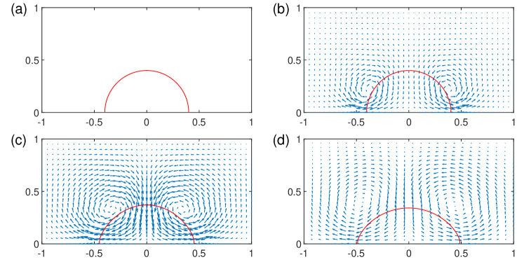
We investigate the detailed dynamics of a droplet on dielectric substrates driven by the electric force. We consider a hydrophilic case with the contact angle θY=π/3\theta_{Y}=\pi/3 and a hydrophobic case with the contact angle θY=2π/3\theta_{Y}=2\pi/3. The initial configuration of the system and the discretizations of the computational domain and the interface are the same as those in the previous example. Several snapshots of the interface profile are shown in Fig. 7 for the hydrophilic case and in Fig. 8 for the hydrophobic case. Also shown in the figures are the respective velocity field. We observe that vortices are generated near the contact points, driving the droplet to spread on the substrate.

In Fig. 9, we plot the loss of the total energy ΔW:=W(t)W(0)\Delta W:=W(t)-W(0) (left panel) and the kinetic energy of the fluids Wk(t)=Ω12ρ|𝐮|2𝑑2W_{k}(t)=\int_{\Omega}\frac{1}{2}\rho|\mathbf{u}|^{2}d\mathcal{L}^{2} (right panel) as functions of time. The total energy, as given in Eq. (21), consists of the kinetic energy, the interfacial energies and the electrostatic energy. We observe that the total energy of the discrete system decays in time, a desired property of the numerical method.

Refer to caption
Fig. 10: Snapshots of the droplet migrating on a dielectric substrate. The electrostatic potential on the lower boundary of the substrate is prescribed as Φ|y=d=38(x+1)\Phi|_{y=-d}=\frac{3}{8}(x+1). Other parameters are η=0.2\eta=0.2, ϵ2=ϵ3=1\epsilon_{2}=\epsilon_{3}=1, d=0.2d=0.2, and θY=2π/3\theta_{Y}=2\pi/3. (a) t=0t=0; (b) t=0.1t=0.1; maxxΩ|𝐮|=0.99\max_{x\in\Omega}|\mathbf{u}|=0.99; (c) t=0.5t=0.5; max𝐱Ω|𝐮|=0.34\max_{\mathbf{x}\in\Omega}|\mathbf{u}|=0.34; (d) t=1.2t=1.2, max𝐱Ω|𝐮|=0.56\max_{\mathbf{x}\in\Omega}|\mathbf{u}|=0.56; (e) t=1.8t=1.8, maxxΩ|𝐮|=0.90\max_{x\in\Omega}|\mathbf{u}|=0.90; (f)t=2.3t=2.3, max𝐱Ω|𝐮|=0.41\max_{\mathbf{x}\in\Omega}|\mathbf{u}|=0.41.

In the last example, we simulate the migration of a droplet on a substrate with non-uniform electrostatic potential prescribed on the boundary. The non-uniform potential mimics an array of electrodes placed below the substrate that is used to transport the droplet in experiments. The electrostatic potential on the lower boundary of the substrate is given as Φ|y=d=38(x+1)\Phi|_{y=-d}=\frac{3}{8}(x+1). Other parameters are chosen as η=0.2\eta=0.2, ϵ2=ϵ3=1\epsilon_{2}=\epsilon_{3}=1, d=0.2d=0.2, and θY=2π/3\theta_{Y}=2\pi/3. The initial interface of the droplet is given by a semi-ellipse as (x0.5)20.32+y20.22=1,y0\frac{(x-0.5)^{2}}{0.3^{2}}+\frac{y^{2}}{0.2^{2}}=1,\;y\geq 0. Numerical results for the interface profile and the velocity field are shown in Fig. 10. We observe that the droplet first de-wets the substrate to form a near-circular shape with contact angle close to θY=2π/3\theta_{Y}=2\pi/3. In this stage, the dynamics is mainly driven by the surface tension. Afterwards, the electric force plays dominant role, and it drives the droplet to migrate from the right to the left.

5 Conclusions

In this work, we presented a hydrodynamic model for electrowetting on dielectric based on the earlier work on moving contact lines, and developed an efficient numerical method for the model. The numerical method combines a semi-implicit parametric finite element method for the dynamics of the fluid interface and the finite element method for the Navier-Stokes equations as well as the boundary integral method for the electric field. We proved that the numerical method admits a unique solution. In the case without the electric field, we showed that the numerical method obeys a similar energy law as the continuum model.

In the numerical experiments, we assessed the accuracy and convergence of the numerical method and investigated the effect of the different physical parameters on the interface dynamics and its equilibrium profile. Numerical results for the equilibrium profile of the interface agree well with the predictions of the Lippmann equation.

The numerical solution for the electric force exhibits a singular structure near the contact point that is consistent with theoretical results. This singularity incurs large curvature of the interface near the contact point, which deteriorates the convergence order of the numerical solution, particularly the convergence of the contact angle to the equilibrium angle.

In this work, we focused on simulations in two dimensions. The numerical method can be readily extended to three-dimensional problems. This will be left to our future work.

Acknowledgement

The work was partially supported by Singapore MOE RSB grant, Singapore MOE AcRF grants (No. R-146-000-267-114, No. R-146-000-285-114) and NSFC grant (No. 11871365).

Appendix A Energy law for the continuum model

The total energy for the EWoD model (3)-(9) in its original dimension form reads

(56) W(t)=i=1,2Ωi12ρi|𝐮|2d2γcosθY|Γ1(t)|+γ|Γ(t)|i=2,3Ωi12ϵi|Φ|2d2.W(t)=\sum_{i=1,2}\int_{\Omega_{i}}\frac{1}{2}\rho_{i}|\mathbf{u}|^{2}{\rm d}{\mathcal{L}}^{2}-\gamma\cos\theta_{Y}|\Gamma_{1}(t)|+\gamma|\Gamma(t)|-\sum_{i=2,3}\int_{\Omega_{i}}\frac{1}{2}\epsilon_{i}|\nabla\Phi|^{2}\;{\rm d}{\mathcal{L}}^{2}.

Integrating by parts and using the electrostatic potential equation in (7) as well as the boundary conditions for Φ\Phi, we can transform the electrical energy in (56) into expressions only involving line integrals over Γ\Gamma and Γ1\Gamma_{1}. This gives the following alternative form of the total energy

W(t)=i=1,2Ωi12ρi|𝐮|2d2γcosθY|Γ1(t)|+γ|Γ(t)|\displaystyle W(t)=\sum_{i=1,2}\int_{\Omega_{i}}\frac{1}{2}\rho_{i}|\mathbf{u}|^{2}{\rm d}{\mathcal{L}}^{2}-\gamma\cos\theta_{Y}|\Gamma_{1}(t)|+\gamma|\Gamma(t)|
(57) +ϕ2(Γϵ2(𝐧Φ)ds+Γ1ϵ3(𝐧wΦ)ds),\displaystyle\quad\qquad\qquad\qquad+\frac{\phi}{2}\left(\int_{\Gamma}\epsilon_{2}\,(\mathbf{n}\cdot\nabla\Phi)\;{\rm d}s+\int_{\Gamma_{1}}\epsilon_{3}\,(\mathbf{n}_{w}\cdot\nabla\Phi)\;{\rm d}s\right),

which can be used to compute the discrete electrical energy in view of the boundary integral method in (41). The dynamic system obeys the energy dissipation law

(58) ddtW(t)=i=1,2Ωi2μiD(𝐮)F2d2i=1,2Γiβi|us|2dsβ(x˙l2+x˙r2)0.\frac{{\rm d}}{{\rm d}t}W(t)=-\sum_{i=1,2}\int_{\Omega_{i}}2\mu_{i}\lVert D(\mathbf{u})\rVert_{F}^{2}{\rm d}{\mathcal{L}}^{2}-\sum_{i=1,2}\int_{\Gamma_{i}}\beta_{i}|u_{s}|^{2}{\rm d}s-\beta^{*}(\dot{x}_{l}^{2}+\dot{x}_{r}^{2})\leq 0.

We show the proof of (58). The dissipation of the fluid kinetic energy is

ddti=1,2Ωi(t)12ρi|𝐮|2d2=i=1,2Ωiρi𝐮(t𝐮+𝐮𝐮)d2\displaystyle\frac{{\rm d}}{{\rm d}t}\sum_{i=1,2}\int_{\Omega_{i}(t)}\frac{1}{2}\rho_{i}|\mathbf{u}|^{2}\;{\rm d}{\mathcal{L}}^{2}=\sum_{i=1,2}\int_{\Omega_{i}}\rho_{i}\mathbf{u}\cdot(\partial_{t}\mathbf{u}+\mathbf{u}\cdot\nabla\mathbf{u})\;{\rm d}{\mathcal{L}}^{2}
=i=1,2Ωi𝐮(p+τd)d2\displaystyle\quad=\sum_{i=1,2}\int_{\Omega_{i}}\mathbf{u}\cdot(-\nabla p+\nabla\cdot\tau_{d})\;{\rm d}{\mathcal{L}}^{2}
=i=1,2Ωi𝐮:τdd2i=1,2Γi𝐮τd𝐧wds+Γ𝐮[p𝐈2τd]12𝐧ds\displaystyle\quad=-\sum_{i=1,2}\int_{\Omega_{i}}\nabla\mathbf{u}:\tau_{d}\;{\rm d}{\mathcal{L}}^{2}-\sum_{i=1,2}\int_{\Gamma_{i}}\mathbf{u}\cdot\tau_{d}\cdot\mathbf{n}_{w}\;{\rm d}s+\int_{\Gamma}\mathbf{u}\cdot[p\mathbf{I}_{2}-\tau_{d}]_{1}^{2}\cdot\mathbf{n}\;{\rm d}s
=i=1,2Ωi2μiD(𝐮)F2d2i=1,2Γiβi|us|2ds\displaystyle\quad=-\sum_{i=1,2}\int_{\Omega_{i}}2\mu_{i}\lVert D(\mathbf{u})\rVert_{F}^{2}\;{\rm d}{\mathcal{L}}^{2}-\sum_{i=1,2}\int_{\Gamma_{i}}\beta_{i}|u_{s}|^{2}\;{\rm d}s
(59) +Γ(γκ+ϵ22|Φ|2)(𝐮𝐧)ds,\displaystyle\qquad\qquad\qquad\qquad+\;\int_{\Gamma}(\gamma\kappa+\frac{\epsilon_{2}}{2}|\nabla\Phi|^{2})(\mathbf{u}\cdot\mathbf{n})\;{\rm d}s,

where we have used the divergence free condition in (3b), the interface conditions in (4a)-(4b), the boundary condition (5), the no-slip boundary condition on the upper wall Γ4\Gamma_{4} and the periodic boundary conditions along Γ3\Gamma_{3}.

The time derivative of the interfacial energies is

ddt(γcosθY|Γ1(t)|+γ|Γ(t)|)\displaystyle\frac{{\rm d}}{{\rm d}t}\Bigl{(}-\gamma\cos\theta_{Y}|\Gamma_{1}(t)|+\gamma|\Gamma(t)|\Bigr{)}
=γcosθY(xr˙xl˙)Γγκvnds+γ(xr˙cosθdrxl˙cosθdl)\displaystyle\quad=-\gamma\cos\theta_{Y}(\dot{x_{r}}-\dot{x_{l}})-\int_{\Gamma}\gamma\kappa\,v_{n}\;{\rm d}s+\gamma\left(\dot{x_{r}}\cos\theta_{d}^{r}-\dot{x_{l}}\cos\theta_{d}^{l}\right)
(60) =Γγκ(𝐮𝐧)dsβ(xr˙2+xl˙2),\displaystyle\quad=-\int_{\Gamma}\gamma\kappa\,(\mathbf{u}\cdot\mathbf{n})\;{\rm d}s-\beta^{*}\left(\dot{x_{r}}^{2}+\dot{x_{l}}^{2}\right),

where we have used (4c) and (6).

Denote by 𝐧^\hat{\mathbf{n}} the outward unit normal vector on the boundary of Ω2\Omega_{2} and Ω3\Omega_{3}. Differentiating the electrical energy yields

ddt(12i=2,3Ωiϵi|Φ|2d2)\displaystyle\frac{{\rm d}}{{\rm d}t}\left(-\frac{1}{2}\sum_{i=2,3}\int_{\Omega_{i}}\epsilon_{i}|\nabla\Phi|^{2}\;{\rm d}{\mathcal{L}}^{2}\right)
=12i=2,3Ωi2ϵiΦ(tΦ)d212i=2,3Ωiϵi|Φ|2(𝐮𝐧^)ds\displaystyle\quad=-\frac{1}{2}\sum_{i=2,3}\int_{\Omega_{i}}2\epsilon_{i}\nabla\Phi\cdot\nabla(\partial_{t}\Phi)\;{\rm d}{\mathcal{L}}^{2}-\frac{1}{2}\sum_{i=2,3}\int_{\partial\Omega_{i}}\epsilon_{i}|\nabla\Phi|^{2}(\mathbf{u}\cdot\hat{\mathbf{n}})\,{\rm d}s
=12i=2,3Ωi2ϵi(tΦΦ)d2+12Γϵ2|Φ|2(𝐮𝐧)ds\displaystyle\quad=-\frac{1}{2}\sum_{i=2,3}\int_{\Omega_{i}}2\epsilon_{i}\nabla\cdot(\partial_{t}\Phi\nabla\Phi)\;{\rm d}{\mathcal{L}}^{2}+\frac{1}{2}\int_{\Gamma}\epsilon_{2}|\nabla\Phi|^{2}(\mathbf{u}\cdot\mathbf{n})\;{\rm d}s
=i=2,3ΩiϵitΦ(Φ𝐧^)ds+12Γϵ2|Φ|2(𝐮𝐧)ds\displaystyle\quad=-\sum_{i=2,3}\int_{\partial\Omega_{i}}\epsilon_{i}\partial_{t}\Phi\,(\nabla\Phi\cdot\hat{\mathbf{n}})\,{\rm d}s+\frac{1}{2}\int_{\Gamma}\epsilon_{2}|\nabla\Phi|^{2}(\mathbf{u}\cdot\mathbf{n})\;{\rm d}s
(61) =12Γϵ2|Φ|2(𝐮𝐧)ds,\displaystyle\quad=-\frac{1}{2}\int_{\Gamma}\epsilon_{2}|\nabla\Phi|^{2}\,(\mathbf{u}\cdot\mathbf{n})\;{\rm d}s,

where the first equality results from the Reynolds transport theorem, the second equality is obtained from (7), the third equality comes from the divergence theorem, and for the last equality, we have used the boundary conditions in (8)-(9), the periodic boundary condition along Γ3Γ6\Gamma_{3}\cup\Gamma_{6} as well as the fact that

(62) tΦ+𝐮Φ=0,onΓΓ1Γ4Γ5.\partial_{t}\Phi+\mathbf{u}\cdot\nabla\Phi=0,\qquad{\rm on}\;\Gamma\cup\Gamma_{1}\cup\Gamma_{4}\cup\Gamma_{5}.

Combining Eqs. (59)-(61), we obtain the energy dissipation law in (58). In terms of the dimensionless variables defined in section 2.3, the energy law in (58) gives Eq. (22) (scaled by ρ1U2L2\rho_{1}U^{2}L^{2}).

Appendix B Proof of Theorem 3.1

It suffices to show that the corresponding homogeneous system has only zero solution. By noting that electric force ϵ2η|Φ|2\epsilon_{2}\eta|\nabla\Phi|^{2} in (37) is explicitly evaluated on Γm\Gamma^{m}, thus we can consider solving the following homogeneous system for (𝐮h,ph,𝐗h,κh)(𝕌h,h,𝕏h,𝕂h)\big{(}\mathbf{u}^{h},~{}p^{h},~{}\mathbf{X}^{h},~{}\kappa^{h}\big{)}\in\big{(}\mathbb{U}^{h},~{}\mathbb{P}^{h},~{}\mathbb{X}^{h},~{}\mathbb{K}^{h}\big{)} such that

12[((ρm+ρm1)𝐮hτ,𝝎h)+(ρm(𝐮m)𝐮h,𝝎h)\displaystyle\frac{1}{2}\Bigl{[}\Bigl{(}\frac{(\rho^{m}+\rho^{m-1})\mathbf{u}^{h}}{\tau},~{}\boldsymbol{\omega}^{h}\Bigr{)}+\Bigl{(}\rho^{m}(\mathbf{u}^{m}\cdot\nabla)\mathbf{u}^{h},~{}\boldsymbol{\omega}^{h}\Bigr{)}
(ρm(𝐮m)𝝎h,𝐮h)](ph,𝝎h)\displaystyle\quad-\;\Bigl{(}\rho^{m}(\mathbf{u}^{m}\cdot\nabla)\boldsymbol{\omega}^{h},~{}\mathbf{u}^{h}\Bigr{)}\Bigr{]}-\Bigl{(}p^{h},~{}\nabla\cdot\boldsymbol{\omega}^{h}\Bigr{)}
+2Re(μmD(𝐮h),D(𝝎h))1We(κh𝐧m,𝝎h)Γm\displaystyle\quad+\frac{2}{Re}\,\Bigl{(}\mu^{m}D(\mathbf{u}^{h}),~{}D(\boldsymbol{\omega}^{h})\Bigr{)}-\;\frac{1}{We}\Bigl{(}\kappa^{h}\,\mathbf{n}^{m},~{}\boldsymbol{\omega}^{h}\Bigr{)}_{\Gamma^{m}}
(63a) +1Rels(βmush,ωsh)Γ1mΓ2m=0,𝝎h𝕌h,\displaystyle\quad+\;\frac{1}{Re\cdot l_{s}}\Bigr{(}\beta^{m}\,u_{s}^{h},~{}\omega_{s}^{h}\Bigr{)}_{\Gamma_{1}^{m}\cup\Gamma_{2}^{m}}=0,\quad\forall\boldsymbol{\omega}^{h}\in\mathbb{U}^{h},
(63b) (𝐮h,ζh)=0,ζhh,\displaystyle\qquad\qquad\Bigl{(}\nabla\cdot\mathbf{u}^{h},~{}\zeta^{h}\Bigr{)}=0,\quad\forall\zeta^{h}\in\mathbb{P}^{h},
(63c) (𝐗hτ𝐧m,ψh)Γmh(𝐮h𝐧m,ψh)Γm=0,ψh𝕂h,\displaystyle\Bigl{(}\frac{\mathbf{X}^{h}}{\tau}\cdot\mathbf{n}^{m},~{}\psi^{h}\Bigr{)}_{\Gamma^{m}}^{h}-\Bigl{(}\mathbf{u}^{h}\cdot\mathbf{n}^{m},~{}\psi^{h}\Bigr{)}_{\Gamma^{m}}=0,\quad\forall\psi^{h}\in\mathbb{K}^{h},
(κh𝐧m,𝒈h)Γmh+(s𝐗h,s𝒈h)Γmh\displaystyle\Bigl{(}\kappa^{h}\,\mathbf{n}^{m},~{}\boldsymbol{g}^{h}\Bigr{)}_{\Gamma^{m}}^{h}+\Bigl{(}\partial_{s}\mathbf{X}^{h},~{}\partial_{s}\boldsymbol{g}^{h}\Bigr{)}_{\Gamma^{m}}^{h}
(63d) +βCaτ[xrhg1h(1)+xlhg1h(0)]=0,𝒈h𝕏h,\displaystyle\qquad\qquad\qquad+\frac{\beta^{*}Ca}{\tau}\Bigl{[}x_{r}^{h}\,g_{1}^{h}(1)+x_{l}^{h}\,g_{1}^{h}(0)\Bigr{]}=0,\quad\forall\boldsymbol{g}^{h}\in\mathbb{X}^{h},

where 𝐗h=(Xh,Yh)T\mathbf{X}^{h}=(X^{h},~{}Y^{h})^{T}, ush=𝐮h𝐭wu_{s}^{h}=\mathbf{u}^{h}\cdot\mathbf{t}_{w}, and xlh:=Xh|α=0x_{l}^{h}:=X^{h}|_{\alpha=0} and xrh:=Xh|α=1x_{r}^{h}:=X^{h}|_{\alpha=1}.

Taking 𝝎h=𝐮h\boldsymbol{\omega}^{h}=\mathbf{u}^{h}, ζh=ph\zeta^{h}=p^{h}, ψh=1Weκh\psi^{h}=\frac{1}{We}\kappa^{h} and 𝒈h=1We𝐗h\boldsymbol{g}^{h}=\frac{1}{We}\mathbf{X}^{h}, then combining these equations yields

(ρm+ρm12𝐮h,𝐮h)+2τRe(μmD(𝐮h),D(𝐮h))+τRels(βmush,ush)Γ1mΓ2m\displaystyle\Bigl{(}\frac{\rho^{m}+\rho^{m-1}}{2}\mathbf{u}^{h},\mathbf{u}^{h}\Bigr{)}+\frac{2\tau}{Re}\Bigl{(}\mu^{m}\,D(\mathbf{u}^{h}),D(\mathbf{u}^{h})\Bigr{)}+\frac{\tau}{Re\cdot l_{s}}\Bigl{(}\beta^{m}\,u_{s}^{h},u_{s}^{h}\Bigr{)}_{\Gamma_{1}^{m}\cup\Gamma_{2}^{m}}
(64) +1We(s𝐗h,s𝐗h)Γmh+βReτ[(xrh)2+(xlh)2]=0.\displaystyle\qquad\qquad+\frac{1}{We}\Bigl{(}\partial_{s}\mathbf{X}^{h},~{}\partial_{s}\mathbf{X}^{h}\Bigr{)}_{\Gamma^{m}}^{h}+\frac{\beta^{*}}{Re\cdot\tau}[(x_{r}^{h})^{2}+(x_{l}^{h})^{2}]=0.

By Korn’s inequality, we have

(65) 𝐮h1C[12((ρm+ρm1)𝐮h,𝐮h)+2τRe(μmD(𝐮h),D(𝐮h))]0,\lVert\mathbf{u}^{h}\rVert_{1}\leq C\Bigl{[}\frac{1}{2}\Bigl{(}(\rho^{m}+\rho^{m-1})\mathbf{u}^{h},~{}\mathbf{u}^{h}\Bigr{)}+\frac{2\tau}{Re}\Bigl{(}\mu^{m}\,D(\mathbf{u}^{h}),~{}D(\mathbf{u}^{h})\Bigr{)}\Bigr{]}\leq 0,

thus we immediately obtain 𝐮h=𝟎\mathbf{u}^{h}=\mathbf{0}. We also have 𝐗h=𝟎\mathbf{X}^{h}=\mathbf{0} by noting xrh=xlh=0x_{r}^{h}=x_{l}^{h}=0. Substituting 𝐗h=𝟎\mathbf{X}^{h}=\mathbf{0} into Eq. (63d), we obtain

(66) (κh𝐧m,𝒈h)Γmh=0,𝒈h𝕏h.\Bigl{(}\kappa^{h}\,\mathbf{n}^{m},~{}\boldsymbol{g}^{h}\Bigr{)}_{\Gamma^{m}}^{h}=0,\qquad\forall\boldsymbol{g}^{h}\in\mathbb{X}^{h}.

Denote 𝐧jm=(nj,1m,nj,2m)T,j=1,2,,JΓ\mathbf{n}_{j}^{m}=(n_{j,1}^{m},~{}n_{j,2}^{m})^{T},\;j=1,2,\cdots,J_{{}_{\Gamma}}. Choosing 𝒈h\boldsymbol{g}^{h} in (66) as

(67) 𝒈h|αj={[𝐡j+1m+𝐡jm)]κh(αj),1jJΓ1,(n1,1mκh(αj),0)T,j=0,(nJΓ,1mκh(αj),0)T,j=JΓ,\left.\boldsymbol{g}^{h}\right|_{\alpha_{j}}=\left\{\begin{array}[]{l}\left[\mathbf{h}_{j+1}^{m}+\mathbf{h}_{j}^{m})\right]^{\perp}\kappa^{h}(\alpha_{j}),\quad 1\leq j\leq J_{{}_{\Gamma}}-1,\vspace{0.15cm}\\ \left(n_{1,1}^{m}\kappa^{h}(\alpha_{j}),~{}0\right)^{T},\quad j=0,\vspace{0.15cm}\\ \left(n_{J_{{}_{\Gamma}},1}^{m}\,\kappa^{h}(\alpha_{j}),~{}0\right)^{T},\quad j=J_{{}_{\Gamma}},\end{array}\right.

and by noting the norm in (39), we obtain

0=\displaystyle 0= (κh(α0))22|𝐡1m|(n1,1m)2+(κh(αJΓ))22|𝐡JΓm|(nJΓ,1m)2\displaystyle\,\frac{(\kappa^{h}(\alpha_{0}))^{2}}{2}|\mathbf{h}_{1}^{m}|(n_{1,1}^{m})^{2}+\frac{(\kappa^{h}(\alpha_{J_{{}_{\Gamma}}}))^{2}}{2}|\mathbf{h}_{J_{{}_{\Gamma}}}^{m}|(n_{J_{{}_{\Gamma}},1}^{m})^{2}
(68) +12j=1JΓ1(κh(αj))2|𝐡jm+𝐡j+1m|2,\displaystyle\qquad+\;\frac{1}{2}\sum_{j=1}^{J_{{}_{\Gamma}}-1}\left(\kappa^{h}(\alpha_{j})\right)^{2}|\mathbf{h}_{j}^{m}+\mathbf{h}_{j+1}^{m}|^{2},

which implies κh(αj)=0,0jJΓ\kappa^{h}(\alpha_{j})=0,\;\forall 0\leq j\leq J_{{}_{\Gamma}} from the assmuptions i)–iii). We then substitute 𝐮h=𝟎\mathbf{u}^{h}=\mathbf{0} and κh=0\kappa^{h}=0 into (63) and obtain

(69) (ph,𝝎h)=0,𝝎h𝕌h.\left(p^{h},~{}\nabla\cdot\boldsymbol{\omega}^{h}\right)=0,\qquad\forall\boldsymbol{\omega}^{h}\in\mathbb{U}^{h}.

Using the stability condition in (35), we consequently obtain ph=0p^{h}=0. This shows that the homogeneous linear system (63) - (63d) has only the zero solution. Thus, the numerical scheme (37)-(37d) admits a unique solution.

Appendix C Proof of Theorem 3.2

Setting 𝝎h=𝐮m+1\boldsymbol{\omega}^{h}=\mathbf{u}^{m+1}, ζh=pm+1\zeta^{h}=p^{m+1}, ψh=1Weκm+1\psi^{h}=\frac{1}{We}\,\kappa^{m+1} and 𝒈h=1Weτ(𝐗m+1𝐗m)\boldsymbol{g}^{h}=\frac{1}{We\cdot\tau}(\mathbf{X}^{m+1}-\mathbf{X}^{m}) in Eqs. (37)-(37d), noting η=0\eta=0 and then combining these equations yield

12τ[(ρm𝐮m+1ρm1𝐮m,𝐮m+1)+(ρm1(𝐮m+1𝐮m),𝐮m+1)]\displaystyle\frac{1}{2\tau}\left[\Bigl{(}\rho^{m}\mathbf{u}^{m+1}-\rho^{m-1}\mathbf{u}^{m},~{}\mathbf{u}^{m+1}\Bigr{)}+\Bigl{(}\rho^{m-1}\left(\mathbf{u}^{m+1}-\mathbf{u}^{m}\right),~{}\mathbf{u}^{m+1}\Bigr{)}\right]
+2Re(μmD(𝐮m+1),D(𝐮m+1))+1Rels(βmusm+1,usm+1)Γ1mΓ2m\displaystyle\qquad+\;\frac{2}{Re}\,\Bigl{(}\mu^{m}D(\mathbf{u}^{m+1}),~{}D(\mathbf{u}^{m+1})\Bigr{)}+\frac{1}{Re\cdot l_{s}}\left(\beta^{m}\,u_{s}^{m+1},~{}u_{s}^{m+1}\right)_{\Gamma_{1}^{m}\cup\Gamma_{2}^{m}}
+1Weτ(s𝐗m+1,s(𝐗m+1𝐗m))Γmh\displaystyle\qquad+\;\frac{1}{We\cdot\tau}\Bigl{(}\partial_{s}\mathbf{X}^{m+1},~{}\partial_{s}(\mathbf{X}^{m+1}-\mathbf{X}^{m})\Bigr{)}_{\Gamma^{m}}^{h}
cosθYWeτ[(xrm+1xlm+1)(xrmxlm)]\displaystyle\qquad-\;\frac{\cos\theta_{Y}}{We\cdot\tau}\left[(x_{r}^{m+1}-x_{l}^{m+1})-(x_{r}^{m}-x_{l}^{m})\right]
(70) +βRe[(xrm+1xrmτ)2+(xlm+1xlmτ)2]=0.\displaystyle\qquad+\;\frac{\beta^{*}}{Re}\left[\left(\frac{x_{r}^{m+1}-x_{r}^{m}}{\tau}\right)^{2}+\left(\frac{x_{l}^{m+1}-x_{l}^{m}}{\tau}\right)^{2}\right]=0.

It is easy to see that the following inequalities hold:

(ρm𝐮m+1ρm1𝐮m,𝐮m+1)+(ρm1(𝐮m+1𝐮m),𝐮m+1)\displaystyle\Bigl{(}\rho^{m}\mathbf{u}^{m+1}-\rho^{m-1}\mathbf{u}^{m},~{}\mathbf{u}^{m+1}\Bigr{)}+\Bigl{(}\rho^{m-1}\left(\mathbf{u}^{m+1}-\mathbf{u}^{m}\right),~{}\mathbf{u}^{m+1}\Bigr{)}
(71) (ρm𝐮m+1,𝐮m+1)(ρm1𝐮m,𝐮m).\displaystyle\qquad\qquad\geq\Bigl{(}\rho^{m}\,\mathbf{u}^{m+1},~{}\mathbf{u}^{m+1}\Bigr{)}-\Bigl{(}\rho^{m-1}\,\mathbf{u}^{m},~{}\mathbf{u}^{m}\Bigr{)}.
(72) (s𝐗m+1,s(𝐗m+1𝐗m))Γmh|Γm+1||Γm|.\displaystyle\Bigl{(}\partial_{s}\mathbf{X}^{m+1},~{}\partial_{s}(\mathbf{X}^{m+1}-\mathbf{X}^{m})\Bigr{)}_{\Gamma^{m}}^{h}\geq|\Gamma^{m+1}|-|\Gamma^{m}|.

Using (71) and (72) in (70) and noting xrm+1xlm+1=|Γ1m+1|x_{r}^{m+1}-x_{l}^{m+1}=|\Gamma_{1}^{m+1}|, xrmxlm=|Γ1m|x_{r}^{m}-x_{l}^{m}=|\Gamma_{1}^{m}|, we immediately obtain Eq. (43). Replacing mm by kk in Eq. (43) and by summarising up for kk from 0 to m1m-1, we obtain the global discrete energy dissipation law (44).

References

  • [1] M. Agnese and R. Nürnberg, Fitted finite element discretization of two-phase Stokes flow, Int J Numer Methods Fluids., 82 (2016), pp. 709–729.
  • [2] J. W. Barrett, H. Garcke, and R. Nürnberg, A parametric finite element method for fourth order geometric evolution equations, J. Comput. Phys., 222 (2007), pp. 441–467.
  • [3] J. W. Barrett, H. Garcke, and R. Nürnberg, A stable parametric finite element discretization of two-phase Navier–Stokes flow, J. Sci. Comput., 63 (2015), pp. 78–117.
  • [4] B. Berge, Electrocapillarité et mouillage de films isolants par l’eau, Comptes Rendus de L’Academie des Sciences Paris, Serie, II, 317 (1993), pp. 157–163.
  • [5] M. Bienia, M. Vallade, C. Quilliet, and F. Mugele, Electrical-field-induced curvature increase on a drop of conducting liquid, Europhys. Lett., 74 (2006), 103.
  • [6] J. Buehrle, S. Herminghaus, and F. Mugele, Interface profiles near three-phase contact lines in electric fields, Phys. Rev. Lett., 91 (2003), 086101.
  • [7] L. Chen and E. Bonaccurso, Electrowetting - from statics to dynamics, Adv. Colloid Interface Sci., 210 (2014), pp. 2–12.
  • [8] S. K. Cho, H. Moon, and C.-J. Kim, Creating, transporting, cutting, and merging liquid droplets by electrowetting-based actuation for digital microfluidic circuits, J. Microelectromechanical. Syst., 12 (2003), pp. 70–80.
  • [9] L. Clime, D. Brassard, and T. Veres, Numerical modeling of electrowetting processes in digital microfluidic devices, Comput & Fluids, 39 (2010), pp. 1510–1515.
  • [10] L. Corson, N. Mottram, B. Duffy, S. Wilson, C. Tsakonas, and C. Brown, Dynamic response of a thin sessile drop of conductive liquid to an abruptly applied or removed electric field, Phys. Rev. E, 94 (2016), 043112.
  • [11] L. T. Corson, C. Tsakonas, B. R. Duffy, N. J. Mottram, I. C. Sage, C. V. Brown, and S. K. Wilson, Deformation of a nearly hemispherical conducting drop due to an electric field: Theory and experiment, Phys. Fluids, 26 (2014), 122106.
  • [12] D. Crowdy, Exact solutions for the static dewetting of two-dimensional charged conducting droplets on a substrate, Phys. Fluids, 27 (2015), 061705.
  • [13] H. Cui and W. Ren, Interface profile near the contact line in electro-wetting on dielectric, SIAM J. Appl. Math., 80 (2020), pp. 402–421.
  • [14] C. D. Daub, D. Bratko, K. Leung, and A. Luzar, Electrowetting at the nanoscale, J. Phys. Chem. C, 111 (2007), pp. 505–509.
  • [15] H. B. Eral, D. M. Augustine, M. H. Duits, and F. Mugele, Suppressing the coffee stain effect: how to control colloidal self-assembly in evaporating drops using electrowetting, Soft Matter, 7 (2011), pp. 4954–4958.
  • [16] M. Fontelos, G. Grün, U. Kindelan, and F. Klingbeil, Numerical simulation of static and dynamic electrowetting, J. Adhes. Sci. Technol., 26 (2012), pp. 1805–1824.
  • [17] Y. Guan, B. Li, and L. Xing, Numerical investigation of electrowetting-based droplet splitting in closed digital microfluidic system: Dynamics, mode, and satellite droplet, Phys. Fluids, 30 (2018), 112001.
  • [18] R. A. Hayes and B. J. Feenstra, Video-speed electronic paper based on electrowetting, Nature, 425 (2003), 383.
  • [19] H. K. Kang, How electrostatic fields change contact angle in electrowetting, Langmuir, 18 (2002), pp. 10318–10322.
  • [20] S. Kuiper and B. Hendriks, Variable-focus liquid lens for miniature cameras, Appl. Phys. Lett., 85 (2004), pp. 1128–1130.
  • [21] A. Kutana and K. Giapis, Atomistic simulations of electrowetting in carbon nanotubes, Nano. Lett., 6 (2006), pp. 656–661.
  • [22] H. Li and H. Fang, Lattice Boltzmann simulation of electrowetting, Euro. Phys. J. Special Topics, 171 (2009), pp. 129–133.
  • [23] G. Lippmann, Relations entre les phénomènes électriques et capillaires, PhD thesis, Gauthier-Villars Paris, France:, 1875.
  • [24] H.-W. Lu, K. Glasner, A. Bertozzi, and C.-J. Kim, A diffuse-interface model for electrowetting drops in a Hele-Shaw cell, J. Fluid. Mech., 590 (2007), pp. 411–435.
  • [25] J. Monnier, P. Witomski, P. Chow-Wing-Bom, and C. Scheid, Numerical modeling of electrowetting by a shape inverse approach, SIAM J. Appl. Math., 69 (2009), pp. 1477–1500.
  • [26] H. Moon, S. K. Cho, R. L. Garrell, and C.-J. C. Kim, Low voltage electrowetting-on-dielectric, J. Appl. Phys., 92 (2002), pp. 4080–4087.
  • [27] F. Mugele and J.-C. Baret, Electrowetting: from basics to applications, J. Phys. Condens. Matter, 17 (2005), R705.
  • [28] F. Mugele and J. Buehrle, Equilibrium drop surface profiles in electric fields, J. Phys. Condens. Matter, 19 (2007), 375112.
  • [29] M. M. Nahar, G. S. Bindiganavane, J. Nikapitiya, and H. Moon, Numerical modeling of 3D electrowetting droplet actuation and cooling of a hotspot, in Proceedings of the 2015 COMSOL Conference, Boston, MA, USA, 2015, pp. 7–9.
  • [30] R. H. Nochetto, A. J. Salgado, and S. W. Walker, A diffuse interface model for electrowetting with moving contact lines, Math. Mod. Meth. Appl. Sci., 24 (2014), pp. 67–111.
  • [31] M. G. Pollack, A. D. Shenderov, and R. B. Fair, Electrowetting-based actuation of droplets for integrated microfluidics, Appl. Phys. Lett., 2 (2002), pp. 96–101.
  • [32] C. Quilliet and B. Berge, Electrowetting: a recent outbreak, Curr. Opin. Colloid Interface Sci., 6 (2001), pp. 34–39.
  • [33] W. Ren and W. E, Boundary conditions for the moving contact line problem, Phys. Fluids, 19 (2007), 022101.
  • [34] W. Ren and W. E, Derivation of continuum models for the moving contact line problem based on thermodynamic principles, Commun. Math. Sci., 9 (2011), pp. 597–606.
  • [35] W. Ren, D. Hu, and W. E, Continuum models for the contact line problem, Phys. Fluids, 22 (2010), 102103.
  • [36] É. Ruiz-Gutiérrez and R. Ledesma-Aguilar, Lattice-Boltzmann simulations of electrowetting phenomena, Langmuir, 35 (2019), pp. 4849–4859.
  • [37] C. Scheid and P. Witomski, A proof of the invariance of the contact angle in electrowetting, Math. Comput. Model., 49 (2009), pp. 647–665.
  • [38] B. Shapiro, H. Moon, R. L. Garrell, and C.-J. C. Kim, Equilibrium behavior of sessile drops under surface tension, applied external fields, and material variations, J. Appl. Phys., 93 (2003), pp. 5794–5811.
  • [39] M. Vallet, M. Vallade, and B. Berge, Limiting phenomena for the spreading of water on polymer films by electrowetting, Eur. Phys. J. B, 11 (1999), pp. 583–591.
  • [40] H. Verheijen and M. Prins, Reversible electrowetting and trapping of charge: model and experiments, Langmuir, 15 (1999), pp. 6616–6620.
  • [41] S. W. Walker and B. Shapiro, Modeling the fluid dynamics of electrowetting on dielectric (EWOD), J. Microelectromech. Syst., 15 (2006), pp. 986–1000.
  • [42] Q. Zhao, W. Jiang, and W. Bao, An energy-stable parametric finite element method for simulating solid-state dewetting, (2020), arXiv:2003.01677 [math.NA].
  • [43] Q. Zhao and W. Ren, An energy-stable finite element method for the simulation for moving contact lines in two-phase flows, J. Comput. Phys., 417 (2020), doi:10.1016/j.jcp.2020.109582.
  • [44] Y.-P. Zhao and Y. Wang, Fundamentals and applications of electrowetting, Rev. Adhes. Adhes., 1 (2013), pp. 114–174.