This paper was converted on www.awesomepapers.org from LaTeX by an anonymous user.
Want to know more? Visit the Converter page.

A Distribution Free Conditional Independence Test with Applications to Causal Discovery

Zhanrui Cai1, Runze Li2, and Yaowu Zhang3
1,2 The Pennsylvania State University, USA
3 Shanghai University of Finance and Economics, China
Abstract

This paper is concerned with test of the conditional independence. We first establish an equivalence between the conditional independence and the mutual independence. Based on the equivalence, we propose an index to measure the conditional dependence by quantifying the mutual dependence among the transformed variables. The proposed index has several appealing properties. (a) It is distribution free since the limiting null distribution of the proposed index does not depend on the population distributions of the data. Hence the critical values can be tabulated by simulations. (b) The proposed index ranges from zero to one, and equals zero if and only if the conditional independence holds. Thus, it has nontrivial power under the alternative hypothesis. (c) It is robust to outliers and heavy-tailed data since it is invariant to conditional strictly monotone transformations. (d) It has low computational cost since it incorporates a simple closed-form expression and can be implemented in quadratic time. (e) It is insensitive to tuning parameters involved in the calculation of the proposed index. (f) The new index is applicable for multivariate random vectors as well as for discrete data. All these properties enable us to use the new index as statistical inference tools for various data. The effectiveness of the method is illustrated through extensive simulations and a real application on causal discovery.

Key words : Conditional independence, mutual independence, distribution free.

1 Introduction

Conditional independence is fundamental in graphical models and causal inference (Jordan, 1998). Under multinormality assumption, conditional independence is equivalent to the corresponding partial correlation being 0. Thus, partial correlation may be used to measure conditional dependence (Lawrance, 1976). However, partial correlation has low power in detecting conditional dependence in the presence of nonlinear dependence. In addition, it cannot control Type I error when the multinormality assumption is violated. In general, testing for conditional independence is much more challenging than for unconditional independence (Zhang et al., 2011; Shah and Peters, 2020).

Recent works on test of conditional independence have focused on developing omnibus conditional independence test without assuming specific functional forms of the dependencies. Linton and Gozalo (1996) proposed a nonparametric conditional independence test based on the generalization of empirical distribution function, and proposed using bootstrap to obtain the null distribution of the proposed test. This diminishes the computational efficiency. Other approaches include measuring the difference between conditional characteristic functions (Su and White, 2007), the weighted Hellinger distance (Su and White, 2008), and the empirical likelihood (Su and White, 2014). Although these authors established the asymptotical normality of the proposed test under conditional independence, the performance of their proposed tests relies heavily on consistent estimate of the bias and variance terms, which are quite complicated in practice. The asymptotical null distribution may perform badly with a small sample. Thus, the authors recommended obtaining critical values of the proposed tests by a bootstrap. This results in heavy computation burdens. Huang (2010) proposed a test of conditional independence based on the maximum nonlinear conditional correlation. By discretizing the conditioning set into a set of bins, the author transforms the original problem into an unconditional testing problem. Zhang et al. (2011) proposed a kernel-based conditional independence test, which essentially tests for zero Hilbert-Schmidt norm of the partial cross-covariance operator in the reproducing kernel Hilbert spaces. The test also required a bootstrap to approximate the null distribution. Wang et al. (2015) introduced the energy statistics into the conditional test and developed the conditional distance correlation based on Székely et al. (2007), which can also be linked to kernel-based approaches. But the test statistics requires to compute high order U–statistics and therefore suffers heavy computation burden, which is of order O(n3)O(n^{3}) for a sample with size nn. Runge (2018) proposed a non-parametric conditional independence testing based on the information theory framework, in which the conditional mutual information was estimated directly via combining the kk-nearest neighbor estimator with a nearest-neighbor local permutation scheme. However, the theoretical distribution of the proposed test is unclear.

In this paper, we develop a new methodology to test conditional independence and propose conditional independence tests that are applicable for continuous or discrete random variables or vectors. Let XX, YY and ZZ be three continuous random variables. We are interested in testing whether XX and YY are statistically independent given ZZ:

H0:XYZ, versus H1: otherwise.\displaystyle H_{0}:X\bot\!\!\!\bot Y\mid Z,\quad\textrm{ versus }\quad H_{1}:\textrm{ otherwise}.

Here we focus on random variables for simplicity. We will consider test of conditional independence for random vectors in Section 3. To begin with, we observe that with Rosenblatt transformation (Rosenblatt, 1952), i.e., U=defFXZ(XZ)U\stackrel{{\scriptstyle\mbox{{\rm\tiny def}}}}{{=}}F_{X\mid Z}(X\mid Z), V=defFYZ(YZ)V\stackrel{{\scriptstyle\mbox{{\rm\tiny def}}}}{{=}}F_{Y\mid Z}(Y\mid Z) and W=defFZ(Z)W\stackrel{{\scriptstyle\mbox{{\rm\tiny def}}}}{{=}}F_{Z}(Z), XYZX\bot\!\!\!\bot Y\mid Z is equivalent to the mutual independence of UU, VV and WW. Thus we convert a conditional independence test into a mutual independence test, and any technique for testing mutual independence can be readily applied. For example, Chakraborty and Zhang (2019) proposed the joint distance covariance to test mutual independence and Drton et al. (2020) constructed a family of tests with maxima of rank correlations in high dimensions. However, these mutual independence tests do not consider the intrinsic properties of UU, VV and WW. This motivates us to develop a new index ρ\rho to measure the mutual dependence. We show that the index ρ\rho has a closed form, which is much simpler than that of Chakraborty and Zhang (2019). In addition, it is symmetric, invariant to strictly monotone transformations, and ranges from zero to one, and is equal to zero if and only if UU, VV and WW are mutually independent. Based on the index ρ\rho, we further proposed tests of conditional independence. We would like to further note a recent work proposed by Zhou et al. (2020), who suggested to simply test whether UU and VV are independent. However, this is not fully equivalent to the conditional independence test and it is unclear what kind of power loss one might have.

The proposed tests have several appealing features. (a) The proposed test is distribution free in the sense that its limiting null distribution does not depend on unknown parameters and the population distributions of the data. The fact that both UU and VV are independent of WW makes the test statistic nn-consistent under the null hypothesis without requiring under-smoothing. In addition, even though the test statistic depends on UU, VV and WW, which needs to be estimated nonparametrically, we show that the test statistic has the same asymptotic properties as the statistics where true UU, VV and WW are directly available. This leads to a distribution free test statistic when further considering that U,VU,V and WW are uniformly distributed. Although some tests in the literature are also distribution free, the asymptotic distributions are either complicated to estimate (e.g., Su and White, 2007) or rely on the Gaussian process, which is not known how to simulate (e.g., Song, 2009) and would require a wild bootstrap method to determine the critical values. Compared with existing ones, the limiting null distribution of the proposed test depends on UU, VV and WW only, and the critical values can be easily obtained by a simulation-based procedure. (b) The proposed test has nontrivial power against all fixed alternatives. The population version of the test statistic ranges from zero to one and equals zero if and only if conditional independence holds. Unlike many testing procedures that are weaker than that for conditional independence (e.g., Song, 2009), the equivalence between conditional independence and mutual independence guarantees that the newly proposed test has nontrivial power against all fixed alternatives. (c) The proposed test is robust since it is invariant to strictly monotone transformations and thus, it is robust to outliers. Furthermore, UU, VV and WW all have bounded support, and therefore it is suitable for handling heavy-tailed data. (d) The proposed test has low computational cost. It is a VV–statistic, and direct calculation requires only O(n2)O(n^{2}) computational complexity. (e) It is insensitive to tuning parameters involved in the test statistics. The test statistics are nn–consistent under the null hypothesis without under-smoothing, and is hence much less sensitive to the bandwidth. The proposed index ρ\rho is extended to continuous random vectors and discrete data in Section 3. All these properties enable us to use the new conditional independence test for various data.

The rest of this paper is organized as follows. In Section 2 we first show the equivalence between conditional independence and mutual independence. We propose a new index to measure the mutual dependence, and derive desirable properties of the proposed index in Section 2.1. We propose an estimator for the new index in Section 2.2. The asymptotic distributions of the proposed estimator under the null hypothesis, global alternative, and local alternative hypothesis are derived in Section 2.2. We extend the new index to the multivariate and discrete cases in Section 3. We conduct numerical comparisons and apply the proposed test to causal discovery in directed acyclic graphs in Section 4. Some final remarks are given in Section 5. We provide some additional simulation results as well as all the technical proofs in the appendix.

2 Methodology

To begin with, we establish an equivalence between conditional independence and mutual independence. In this section, we focus on the setting in which XX, YY and ZZ are continuous univariate random variables, and the problem of interest is to test XYZX\bot\!\!\!\bot Y\mid Z. Throughout this section, denote U=FXZ(XZ)U=F_{X\mid Z}(X\mid Z), V=FYZ(YZ)V=F_{Y\mid Z}(Y\mid Z) and W=FZ(Z)W=F_{Z}(Z). The proposed methodology is built upon the following proposition.

Proposition 1

Suppose that XX and YY are both univariate and have continuous conditional distribution functions for every given value of ZZ, and ZZ is a continuous univariate random variable. Then XYZX\bot\!\!\!\bot Y\mid Z if and only if U,U, VV and WW are mutually independent.

We provide a detailed proof of Proposition 1 in the appendix. Essentially, it establishes an equivalence between the conditional independence of XYZX\bot\!\!\!\bot Y\mid Z and the mutual independence among UU, VV and WW under the conditions in Proposition 1. Therefore, we can alleviate the hardness issue of conditional independence testing (Shah and Peters, 2020) by restricting the distribution family of the data such that UU, VV and WW can be estimated sufficiently well using samples. As shown in our theoretical analysis, we further impose certain smoothness conditions on the conditional distributions of X,YZ=zX,Y\mid Z=z as zz varies in the support of ZZ. This distribution family is also considered in Neykov et al. (2020) to develop a minimax optimal conditional independence test. We discuss the extension of Proposition 1 to multivariate and discrete data in Section 3.

According to Proposition 1, any techniques for testing mutual independence among three random variables can be readily applied for conditional independence testing problems. For example, Chakraborty and Zhang (2019) proposed the joint distance covariance and Patra et al. (2016) developed a bootstrap procedure to test mutual independence with known marginals. However, a direct application of these metrics may not be a good choice because it ignores the fact that the variables UU, VV and WW are all uniformly distributed, as well as UWU\bot\!\!\!\bot W and VWV\bot\!\!\!\bot W. Next, we discuss how to develop a new mutual independence test while considering these intrinsic properties of (U,V,W)(U,V,W).

2.1 A mutual independence test

In this section, we propose to characterize the conditional dependence of XX and YY given ZZ through quantifying the mutual dependence among UU, VV and WW. Although our proposed test is based on the distance between characteristics functions, our proposed test is much simpler and has different asymptotic distribution as well as different convergence rate from the conditional distance correlation proposed by Wang et al. (2015). Let ω()\omega(\cdot) be an arbitrary positive weight function and φU,V,W()\varphi_{U,V,W}(\cdot), φU()\varphi_{U}(\cdot), φV()\varphi_{V}(\cdot), and φW()\varphi_{W}(\cdot) be the characteristic functions of (U,V,W)(U,V,W), UU, VV and WW, respectively. Then

UU, VV and WW are mutually independent
\displaystyle\Longleftrightarrow φU,V,W(t1,t2,t3)=φU(t1)φV(t2)φW(t3) for all t1,t2,t3\displaystyle\varphi_{U,V,W}(t_{1},t_{2},t_{3})=\varphi_{U}(t_{1})\varphi_{V}(t_{2})\varphi_{W}(t_{3})\textrm{ for all $t_{1},t_{2},t_{3}\in\mathbb{R}$}
\displaystyle\Longleftrightarrow φU,V,W(t1,t2,t3)φU(t1)φV(t2)φW(t3)2ω(t1,t2,t3)𝑑t1𝑑t2𝑑t3=0,\displaystyle\iiint\big{\|}\varphi_{U,V,W}(t_{1},t_{2},t_{3})-\varphi_{U}(t_{1})\varphi_{V}(t_{2})\varphi_{W}(t_{3})\big{\|}^{2}\omega(t_{1},t_{2},t_{3})dt_{1}dt_{2}dt_{3}=0,

where ψ2=ψTψ¯\|\psi\|^{2}=\psi^{\mbox{\tiny{T}}}\overline{\psi} for a complex-valued function ψ\psi and ψ¯\overline{\psi} is the conjugate of ψ\psi. By choosing ω(t1,t2,t3)\omega(t_{1},t_{2},t_{3}) to be the joint probability density function of three independent and identically distributed standard Cauchy random variables, the integration in the above equation has a closed form,

Ee|U1U2||V1V2||W1W2|2Ee|U1U3||V1V4||W1W2|\displaystyle Ee^{-|U_{1}-U_{2}|-|V_{1}-V_{2}|-|W_{1}-W_{2}|}-2Ee^{-|U_{1}-U_{3}|-|V_{1}-V_{4}|-|W_{1}-W_{2}|}
+Ee|U1U2|Ee|V1V2|Ee|W1W2|,\displaystyle\hskip 85.35826pt+Ee^{-|U_{1}-U_{2}|}Ee^{-|V_{1}-V_{2}|}Ee^{-|W_{1}-W_{2}|}, (1)

where (Uk,Vk,Wk)(U_{k},V_{k},W_{k}), k=1,,4k=1,\ldots,4, are four independent copies of (U,V,W)(U,V,W). Here the choice of the weight function ω(t1,t2,t3)\omega(t_{1},t_{2},t_{3}) is mainly for the convenient analytic form of the integration. Different from the distance correlation (Székely et al., 2007), our integration exists without any moment conditions on the data, which is more widely applicable. Furthermore, with the fact that UWU\bot\!\!\!\bot W and VWV\bot\!\!\!\bot W, (1) boils down to

E{SU(U1,U2)SV(V1,V2)e|W1W2|},\displaystyle E\left\{S_{U}(U_{1},U_{2})S_{V}(V_{1},V_{2})e^{-|W_{1}-W_{2}|}\right\}, (2)

where SU(U1,U2)S_{U}(U_{1},U_{2}) and SV(V1,V2)S_{V}(V_{1},V_{2}) are defined as

SU(U1,U2)\displaystyle S_{U}(U_{1},U_{2}) =\displaystyle= E{e|U1U2|+e|U3U4|e|U1U3|e|U2U3|(U1,U2)},\displaystyle E\left\{e^{-|U_{1}-U_{2}|}+e^{-|U_{3}-U_{4}|}-e^{-|U_{1}-U_{3}|}-e^{-|U_{2}-U_{3}|}\mid(U_{1},U_{2})\right\},
SV(V1,V2)\displaystyle S_{V}(V_{1},V_{2}) =\displaystyle= E{e|V1V2|+e|V3V4|e|V1V3|e|V2V3|(V1,V2)}.\displaystyle E\left\{e^{-|V_{1}-V_{2}|}+e^{-|V_{3}-V_{4}|}-e^{-|V_{1}-V_{3}|}-e^{-|V_{2}-V_{3}|}\mid(V_{1},V_{2})\right\}.

Recall that UU, VV and WW are uniformly distributed on (0,1)(0,1). With further calculations based on (2), we obtain a normalized index and define it as ρ\rho to measure the mutual dependence:

ρ(X,YZ)\displaystyle\rho(X,Y\mid Z) =\displaystyle= c0E{(e|U1U2|+eU1+eU11+eU2+eU21+2e14)\displaystyle c_{0}E\big{\{}\left(e^{-|U_{1}-U_{2}|}+e^{-U_{1}}+e^{U_{1}-1}+e^{-U_{2}}+e^{U_{2}-1}+2e^{-1}-4\right) (3)
(e|V1V2|+eV1+eV11+eV2+eV21+2e14)e|W1W2|},\displaystyle\left(e^{-|V_{1}-V_{2}|}+e^{-V_{1}}+e^{V_{1}-1}+e^{-V_{2}}+e^{V_{2}-1}+2e^{-1}-4\right)e^{-|W_{1}-W_{2}|}\big{\}},

where c0=(13e340e2+13e1)1c_{0}=(13e^{-3}-40e^{-2}+13e^{-1})^{-1}. Several appealing properties of the proposed index ρ(X,YZ)\rho(X,Y\mid Z) are summarized in Theorem 1.

Theorem 1

Suppose that the conditions in Proposition 1 are fulfilled. The index ρ(X,YZ)\rho(X,Y\mid Z) defined in (3) has the following properties:

(1) 0ρ(X,YZ)10\leq\rho(X,Y\mid Z)\leq 1, ρ(X,YZ)=0\rho(X,Y\mid Z)=0 holds if and only if XYZX\bot\!\!\!\bot Y\mid Z. Furthermore, if FX|Z(X|Z)=FY|Z(Y|Z)F_{X|Z}(X|Z)=F_{Y|Z}(Y|Z) or FX|Z(X|Z)+FY|Z(Y|Z)=1F_{X|Z}(X|Z)+F_{Y|Z}(Y|Z)=1, then ρ(X,YZ)=1\rho(X,Y\mid Z)=1.

(2) The index ρ\rho is symmetric conditioning on ZZ. That is, ρ(X,YZ)=ρ(Y,XZ)\rho(X,Y\mid Z)=\rho(Y,X\mid Z).

(3) For any strictly monotone transformations m1()m_{1}(\cdot), m2()m_{2}(\cdot) and m3()m_{3}(\cdot), ρ(X,YZ)=ρ{m1(X),m2(Y)m3(Z)}\rho(X,Y\mid Z)=\rho\left\{m_{1}(X),m_{2}(Y)\mid m_{3}(Z)\right\}.

The step-by-step derivation of ρ(X,YZ)\rho(X,Y\mid Z) and proof of Theorem 1 are presented in the appendix. Property (1) indicates that the index ρ\rho ranges from zero to one, equals zero when the conditional independence holds, and is equal to one if YY is a strictly monotone transformation of XX conditional on ZZ. Property (2) shows that the index ρ\rho is a symmetric measure of conditional dependence. Property (3) illustrates that the index ρ\rho is invariant to any strictly monotone transformation. In fact, ρ\rho is not only invariant to marginal strictly monotone transformations, but also invariant to strictly monotone transformations conditional on ZZ. For example, it can be verified that ρ(X,YZ)=ρ[m1{XE(XZ)},YZ]\rho(X,Y\mid Z)=\rho[m_{1}\{X-E(X\mid Z)\},Y\mid Z].

2.2 Asymptotic properties

In this section, we establish the asymptotic properties of the sample version of the proposed index under the null and alternative hypothesis. Consider independent and identically distributed samples {Xi,Yi,Zi}\{X_{i},Y_{i},Z_{i}\}, i=1,,ni=1,\dots,n. To estimate the proposed index ρ(X,YZ)\rho(X,Y\mid Z), we apply kernel estimator for the conditional cumulative distribution function. Specifically, define

f^Z(z)=n1i=1nKh(zZi),\displaystyle\widehat{f}_{Z}(z)=n^{-1}\sum_{i=1}^{n}K_{h}(z-Z_{i}),
U^=F^XZ(xz)=n1i=1nKh(zZi)𝟙(Xix)/f^Z(z),\displaystyle\widehat{U}=\widehat{F}_{X\mid Z}(x\mid z)=n^{-1}\sum_{i=1}^{n}K_{h}(z-Z_{i})\mathbbm{1}(X_{i}\leq x)/\widehat{f}_{Z}(z),
V^=F^YZ(yz)=n1i=1nKh(zZi)𝟙(Yiy)/f^Z(z),\displaystyle\widehat{V}=\widehat{F}_{Y\mid Z}(y\mid z)=n^{-1}\sum_{i=1}^{n}K_{h}(z-Z_{i})\mathbbm{1}(Y_{i}\leq y)/\widehat{f}_{Z}(z),

where Kh()=K(/h)/hK_{h}(\cdot)=K(\cdot/h)/h, K()K(\cdot) is a kernel function, and hh is the bandwidth. Besides, we use empirical distribution function to estimate the cumulative distribution function, i.e., W^=F^Z(z)=n1i=1n𝟙(Ziz)\widehat{W}=\widehat{F}_{Z}(z)=n^{-1}\sum_{i=1}^{n}\mathbbm{1}(Z_{i}\leq z). The sample version of the index, denoted by ρ^(X,YZ)\widehat{\rho}(X,Y\mid Z), is thus given by

ρ^(X,YZ)\displaystyle\widehat{\rho}(X,Y\mid Z) =\displaystyle= c0n2i,j{(e|U^iU^j|+eU^i+eU^i1+eU^j+eU^j1+2e14)\displaystyle c_{0}n^{-2}\sum_{i,j}\left\{\left(e^{-|\widehat{U}_{i}-\widehat{U}_{j}|}+e^{-\widehat{U}_{i}}+e^{\widehat{U}_{i}-1}+e^{-\widehat{U}_{j}}+e^{\widehat{U}_{j}-1}+2e^{-1}-4\right)\right.
(e|V^iV^j|+eV^i+eV^i1+eV^j+eV^j1+2e14)e|W^iW^j|}.\displaystyle\left.\left(e^{-|\widehat{V}_{i}-\widehat{V}_{j}|}+e^{-\widehat{V}_{i}}+e^{\widehat{V}_{i}-1}+e^{-\widehat{V}_{j}}+e^{\widehat{V}_{j}-1}+2e^{-1}-4\right)e^{-|\widehat{W}_{i}-\widehat{W}_{j}|}\right\}.

One can also obtain a normalized index ρ0\rho_{0}, which is a direct normalization based on (1) without considering UWU\bot\!\!\!\bot W and VWV\bot\!\!\!\bot W:

ρ0(X,YZ)\displaystyle{\rho}_{0}(X,Y\mid Z) =\displaystyle= c0{Ee|U1U2||V1V2||W1W2|+8e3\displaystyle c_{0}\left\{Ee^{-|U_{1}-U_{2}|-|V_{1}-V_{2}|-|W_{1}-W_{2}|}+8e^{-3}\right.
2E(2eU1eU11)(2eV1eV11)(2eW1eW11)}.\displaystyle\left.-2E\left(2-e^{-U_{1}}-e^{U_{1}-1}\right)\left(2-e^{-V_{1}}-e^{V_{1}-1}\right)\left(2-e^{-W_{1}}-e^{W_{1}-1}\right)\right\}.

The corresponding moment estimator is

ρ^0(X,YZ)\displaystyle\widehat{\rho}_{0}(X,Y\mid Z) =\displaystyle= c0{n2i,je|U^iU^j||V^iV^j||W^iW^j|+8e3\displaystyle c_{0}\left\{n^{-2}\sum_{i,j}e^{-|\widehat{U}_{i}-\widehat{U}_{j}|-|\widehat{V}_{i}-\widehat{V}_{j}|-|\widehat{W}_{i}-\widehat{W}_{j}|}+8e^{-3}\right.
2n1i=1n(2eU^ieU^i1)(2eV^ieV^i1)(2eW^ieW^i1)}.\displaystyle\left.-2n^{-1}\sum_{i=1}^{n}\left(2-e^{-\widehat{U}_{i}}-e^{\widehat{U}_{i}-1}\right)\left(2-e^{-\widehat{V}_{i}}-e^{\widehat{V}_{i}-1}\right)\left(2-e^{-\widehat{W}_{i}}-e^{\widehat{W}_{i}-1}\right)\right\}.

Although ρ(X,YZ)=ρ0(X,YZ)\rho(X,Y\mid Z)=\rho_{0}(X,Y\mid Z) at the population level, those two statistics ρ^(X,YZ)\widehat{\rho}(X,Y\mid Z) and ρ^0(X,YZ)\widehat{\rho}_{0}(X,Y\mid Z) exhibit different properties at the sample level. This is because ρ^(X,YZ)\widehat{\rho}(X,Y\mid Z) considers the fact that UWU\bot\!\!\!\bot W and VWV\bot\!\!\!\bot W. But on the other hand, ρ^0(X,YZ)\widehat{\rho}_{0}(X,Y\mid Z) is only a regular mutual independence test statistic, where U^i\widehat{U}_{i}, V^i\widehat{V}_{i}, and W^i\widehat{W}_{i} are exchangeable. When XYZX\bot\!\!\!\bot Y\mid Z, under Conditions 1-4 listed below, ρ^(X,YZ)\widehat{\rho}(X,Y\mid Z) is of order (n1+h4m)(n^{-1}+h^{4m}), while ρ^0(X,YZ)\widehat{\rho}_{0}(X,Y\mid Z) is of order (n1+h2m)(n^{-1}+h^{2m}) because of the bias caused by nonparametric estimation. Note that mm is the order of kernel functions and equal to 2 when using regular kernel functions such as Gaussian and epanechnikov kernels. This indicates that ρ^(X,YZ)\widehat{\rho}(X,Y\mid Z) is essentially nn consistent without under-smoothing while ρ^0(X,YZ)\widehat{\rho}_{0}(X,Y\mid Z) typically requires under-smoothing. In addition, our statistic ρ^(X,YZ)\widehat{\rho}(X,Y\mid Z) has the same asymptotic properties as if U,VU,V and WW are observed, but ρ^0(X,YZ)\widehat{\rho}_{0}(X,Y\mid Z) does not. See Figure 1 for a numerical comparison between the empirical null distributions of the two statistics.

We next study the asymptotical behaviors of the estimated index, ρ^(X,YZ)\widehat{\rho}(X,Y\mid Z), under both the null and the alternative hypotheses. The following regularity conditions are imposed to facilitate our subsequent theoretical analyses. In what follows, we derive the limiting distribution of ρ^(X,YZ)\widehat{\rho}(X,Y\mid Z) under the null hypothesis in Theorem 2.

Condition 1. The univariate kernel function K()K(\cdot) is symmetric about zero and Lipschitz continuous. In addition, it satisfies

K(υ)𝑑υ=1,υiK(υ)𝑑υ=0,1im1,0υmK(υ)𝑑υ<.\displaystyle\int K(\upsilon)d\upsilon=1,\quad\int\upsilon^{i}K(\upsilon)d\upsilon=0,1\leq i\leq m-1,\quad 0\neq\int\upsilon^{m}K(\upsilon)d\upsilon<\infty.

Condition 2. The bandwidth hh satisfies nh2/log2(n)nh^{2}/\log^{2}(n)\to\infty, and nh4m0nh^{4m}\to 0.

Condition 3. The probability density function of ZZ, denoted by fZ(z)f_{Z}(z) is bounded away from 0 to infinity.

Condition 4. The (m1)(m-1)th derivatives of FXZ(xz)f(z)F_{X\mid Z}(x\mid z)f(z), FYZ(yz)f(z)F_{Y\mid Z}(y\mid z)f(z) and fZ(z)f_{Z}(z) with respect to zz are locally Lipschitz-continuous.

Theorem 2

Suppose that Conditions 1-4 hold and the conditions in Proposition 1 are fulfilled. Under the null hypothesis,

nρ^(X,YZ)c0j=1λjχj2(1),\displaystyle n\widehat{\rho}(X,Y\mid Z)\to c_{0}\sum_{j=1}^{\infty}\lambda_{j}\chi_{j}^{2}(1),

in distribution, where χj2(1)\chi_{j}^{2}(1), j=1,2,j=1,2,\dots are independent chi-square random variables with one degree of freedom, and λj\lambda_{j}s, j=1,2,j=1,2,\ldots are eigenvalues of

h(u,v,w;u,v,w)=\displaystyle h(u,v,w;u^{\prime},v^{\prime},w^{\prime})= (e|uu|+eu+eu1+eu+eu1+2e14)(e|vv|\displaystyle(e^{-|u-u^{\prime}|}+e^{-u}+e^{u-1}+e^{-u^{\prime}}+e^{u^{\prime}-1}+2e^{-1}-4)(e^{-|v-v^{\prime}|}
+ev+ev1+ev+ev1+2e14)e|ww|.\displaystyle+e^{-v}+e^{v-1}+e^{-v^{\prime}}+e^{v^{\prime}-1}+2e^{-1}-4)e^{-|w-w^{\prime}|}.

That is, there exists orthonormal eigenfunction Φj(u,v,w)\Phi_{j}(u,v,w) such that

010101h(u,v,w;u,v,w)Φj(u,v,w)𝑑u𝑑v𝑑w=λjΦj(u,v,w).\displaystyle\int_{0}^{1}\int_{0}^{1}\int_{0}^{1}h(u,v,w;u^{\prime},v^{\prime},w^{\prime})\Phi_{j}(u^{\prime},v^{\prime},w^{\prime})du^{\prime}dv^{\prime}dw^{\prime}=\lambda_{j}\Phi_{j}(u,v,w).

The proof of Theorem 2 is given in the appendix. To understand the asymptotic distributions intuitively, we showed in the proof that nρ^(X,YZ)n\widehat{\rho}(X,Y\mid Z) can be approximated by degenerate V-statistics, i.e.,

nρ^(X,YZ)=c0n1i,jh(Ui,Vi,Wi;Uj,Vj,Wj)+op(n1),n\widehat{\rho}(X,Y\mid Z)=c_{0}n^{-1}\sum_{i,j}h(U_{i},V_{i},W_{i};U_{j},V_{j},W_{j})+o_{p}(n^{-1}),

and E{h(Ui,Vi,Wi;Uj,Vj,Wj)(Ui,Vi,Wi)}=0E\{h(U_{i},V_{i},W_{i};U_{j},V_{j},W_{j})\mid(U_{i},V_{i},W_{i})\}=0. By the spectral decomposition,

h(u,v,w;u,v,w)=j=1λjΦj(u,v,w)Φj(u,v,w).h(u,v,w;u^{\prime},v^{\prime},w^{\prime})=\sum_{j=1}^{\infty}\lambda_{j}\Phi_{j}(u,v,w)\Phi_{j}(u^{\prime},v^{\prime},w^{\prime}).

Therefore, nρ^(X,YZ)=c0j=1λj{n1/2i=1nΦj(Ui,Vi,Wi)}2+op(n1),n\widehat{\rho}(X,Y\mid Z)=c_{0}\sum_{j=1}^{\infty}\lambda_{j}\{n^{-1/2}\sum_{i=1}^{n}\Phi_{j}(U_{i},V_{i},W_{i})\}^{2}+o_{p}(n^{-1}), which converges in distribution to the weighted sum of independent chi squared distributions provided in Theorem 2 because n1/2i=1nΦj(Ui,Vi,Wi)n^{-1/2}\sum_{i=1}^{n}\Phi_{j}(U_{i},V_{i},W_{i}) is asymptotically standard normal (Korolyuk and Borovskich, 2013). Moreover, the λj\lambda_{j}s, j=1,2,j=1,2,\dots are real numbers associated with the distribution of UU, VV and WW, all of which follow uniform distributions on [0,1][0,1]. In addition, UU, VV and WW are mutually independent under the null hypothesis. This indicates that the proposed test statistic is essentially distribution free under the null hypothesis. Therefore, we suggest a simulation procedure to approximate the null distribution and decide the critical value. The simulation procedure can be independent of the original data and hence greatly improved the computation efficiency. In what follows, we describe the simulation-based procedure in detail to decide the critical value cαc_{\alpha}.

  1. 1.

    Generate {Ui,Vi,Wi}\{U_{i}^{*},V_{i}^{*},W_{i}^{*}\}, i=1,,ni=1,\dots,n independently from mutually independent standard uniform distributions;

  2. 2.

    Compute the statistic ρ^\widehat{\rho^{*}} based on {Ui,Vi,Wi}\{U_{i}^{*},V_{i}^{*},W_{i}^{*}\}, i=1,,ni=1,\dots,n, i.e.,

    ρ^\displaystyle\widehat{\rho^{*}} =\displaystyle= c0n2i,j{(e|UiUj|+eUi+eUi1+eUj+eUj1+2e14)\displaystyle c_{0}n^{-2}\sum_{i,j}\left\{\left(e^{-|U_{i}^{*}-U_{j}^{*}|}+e^{-U_{i}^{*}}+e^{U_{i}^{*}-1}+e^{-U_{j}^{*}}+e^{U_{j}^{*}-1}+2e^{-1}-4\right)\right.\hskip 65.44142pt (4)
    (e|ViVj|+eVi+eVi1+eVj+eVj1+2e14)e|WiWj|}.\displaystyle\left.\left(e^{-|V_{i}^{*}-V_{j}^{*}|}+e^{-V_{i}^{*}}+e^{V_{i}^{*}-1}+e^{-V_{j}^{*}}+e^{V_{j}^{*}-1}+2e^{-1}-4\right)e^{-|W_{i}^{*}-W_{j}^{*}|}\right\}.
  3. 3.

    Repeat Steps 1-2 for BB times and set cαc_{\alpha} to be the upper α\alpha quantile of the estimated ρ^\widehat{\rho^{*}} obtained from the randomly simulated samples.

Because (U,V,W)(U^{*},V^{*},W^{*}) has the same distribution as that of (U,V,W)(U,V,W) under the null hypothesis, it is straightforward that this simulation-based procedure can provide a valid approximation of the asymptotic null distribution of ρ^(X,YZ)\widehat{\rho}(X,Y\mid Z) when BB is large. The consistency of this procedure is guaranteed by Theorem 3.

Theorem 3

Under Conditions 1-4, it follows that

nρ^c0j=1λjχj2(1)\displaystyle n\widehat{\rho^{*}}\to c_{0}\sum_{j=1}^{\infty}\lambda_{j}\chi_{j}^{2}(1)

in distribution, where χj2(1)\chi_{j}^{2}(1), j=1,2,j=1,2,\dots are independent χ2(1)\chi^{2}(1) variables, and λj\lambda_{j}, j=1,2,j=1,2,\dots are the same as that of Theorem 2.

Next, we study the power performance of the proposed test under two kinds of alternative hypotheses, under which the conditional independence no longer holds. We first consider the global alternative, denoted by H1gH_{1g}, we have

H1g:XYZ.\displaystyle H_{1g}:\quad X\not\!\perp\!\!\!\perp Y\mid Z.

We then consider a sequence of local alternatives, denoted by H1lH_{1l},

H1l:FXZ(xZ=z)FX(Y,Z){x(Y=y,Z=z)}=n1/2(x,y,z).\displaystyle H_{1l}:\quad F_{X\mid Z}(x\mid Z=z)-F_{X\mid(Y,Z)}\left\{x\mid(Y=y,Z=z)\right\}=n^{-1/2}\ell(x,y,z).

The asymptotical properties of the test statistics ρ^(X,YZ)\widehat{\rho}(X,Y\mid Z) under the global alternative and local alternatives are given in Theorem 4, whose proof is in the appendix. Theorem 4 shows that the proposed test can consistently detect any fixed alternatives as well as local alternatives at rate O(n1/2)O(n^{-1/2}).

Theorem 4

Suppose that Conditions 1-4 hold and the conditions in Proposition 1 are fulfilled. Under H1gH_{1g}, when nh2m0nh^{2m}\to 0,

n1/2{ρ^(X,YZ)ρ(X,YZ)}𝒩(0,σ02),\displaystyle n^{1/2}\left\{\widehat{\rho}(X,Y\mid Z)-{\rho}(X,Y\mid Z)\right\}\to\mathcal{N}(0,\sigma^{2}_{0}),

in distribution, where σ02=def4c02var(P1,1+P2,1+P3,1+P4,1)\sigma_{0}^{2}\stackrel{{\scriptstyle\mbox{{\rm\tiny def}}}}{{=}}4c_{0}^{2}\mbox{\rm var}(P_{1,1}+P_{2,1}+P_{3,1}+P_{4,1}), and (P1,1,P2,1,P3,1,P4,1)(P_{1,1},P_{2,1},P_{3,1},P_{4,1}) are defined in (7)-(10) in the appendix, respectively.

Under H1lH_{1l},

nρ^(X,YZ)ζ(t1,t2,t3)2ω(t1,t2,t3)𝑑t1𝑑t2𝑑t3,\displaystyle n\widehat{\rho}(X,Y\mid Z)\to\iiint\left\|\zeta(t_{1},t_{2},t_{3})\right\|^{2}\omega(t_{1},t_{2},t_{3})dt_{1}dt_{2}dt_{3},

in distribution, where ζ(t1,t2,t3)\zeta(t_{1},t_{2},t_{3}) stands for a complex-valued Gaussian random process with mean function E[it1(X,Y,Z)eit1U{eit2VφV(t2)}eit3W]E\left[it_{1}\ell(X,Y,Z)e^{it_{1}U}\left\{e^{it_{2}V}-\varphi_{V}(t_{2})\right\}e^{it_{3}W}\right] and covariance function defined in (11) in the appendix, and ω(t1,t2,t3)\omega(t_{1},t_{2},t_{3}) is the joint probability density function of three independent and identically distributed standard Cauchy random variables.

3 Extensions

3.1 Multivariate continuous data

The methodology developed in Section 2 assumes that all the variables are univariate. In this section, we generalize the proposed index ρ\rho to the multivariate case. Let 𝐱=(X1,,Xp)Tp{\bf x}=(X_{1},\ldots,X_{p})^{\mbox{\tiny{T}}}\in\mathbb{R}^{p}, 𝐲=(Y1,,Yq)Tq{\bf y}=(Y_{1},\ldots,Y_{q})^{\mbox{\tiny{T}}}\in\mathbb{R}^{q} and 𝐳=(Z1,,Zr)Tr{\bf z}=(Z_{1},\ldots,Z_{r})^{\mbox{\tiny{T}}}\in\mathbb{R}^{r} be continuous random vectors. More specifically, all elements of 𝐱{\bf x}, 𝐲{\bf y} and 𝐳{\bf z} are continuous random variables. Define FX1𝐳(X1𝐳)F_{X_{1}\mid{\bf z}}(X_{1}\mid{\bf z}) for the cumulative distribution function of X1X_{1} given 𝐳{\bf z} and FXk𝐳,X1,,Xk1(Xk𝐳,X1,,Xk1)F_{X_{k}\mid{\bf z},X_{1},\ldots,X_{k-1}}(X_{k}\mid{\bf z},X_{1},\ldots,X_{k-1}) for the cumulative distribution function of XkX_{k} given 𝐳,X1,,Xk1{\bf z},X_{1},\ldots,X_{k-1} for k=2,,pk=2,\cdots,p. Similar notation apply for 𝐲{\bf y} and 𝐳{\bf z}. Denote U~1=FX1𝐳(X1𝐳)\widetilde{U}_{1}=F_{X_{1}\mid{\bf z}}(X_{1}\mid{\bf z}), V~1=FY1𝐳(Y1𝐳)\widetilde{V}_{1}=F_{Y_{1}\mid{\bf z}}(Y_{1}\mid{\bf z}), W~1=FZ1(Z1)\widetilde{W}_{1}=F_{Z_{1}}(Z_{1}),

U~k=FXk𝐳,X1,,Xk1(Xk𝐳,X1,,Xk1),k=2,,p,\displaystyle\widetilde{U}_{k}=F_{X_{k}\mid{\bf z},X_{1},\ldots,X_{k-1}}(X_{k}\mid{\bf z},X_{1},\ldots,X_{k-1}),\ k=2,\ldots,p,
V~k=FYk𝐳,Y1,,Yk1(Yk𝐳,Y1,,Yk1),k=2,,q,\displaystyle\widetilde{V}_{k}=F_{Y_{k}\mid{\bf z},Y_{1},\ldots,Y_{k-1}}(Y_{k}\mid{\bf z},Y_{1},\ldots,Y_{k-1}),\ k=2,\ldots,q,
W~k=FZkZ1,,Zk1(ZkZ1,,Zk1),k=2,,r.\displaystyle\widetilde{W}_{k}=F_{Z_{k}\mid Z_{1},\ldots,Z_{k-1}}(Z_{k}\mid Z_{1},\ldots,Z_{k-1}),\ k=2,\ldots,r.

Further denote 𝐮=(U~1,,U~p)T{\bf u}=(\widetilde{U}_{1},\ldots,\widetilde{U}_{p})^{\mbox{\tiny{T}}}, 𝐯=(V~1,,V~q)T{\bf v}=(\widetilde{V}_{1},\ldots,\widetilde{V}_{q})^{\mbox{\tiny{T}}}, 𝐰=(W~1,,W~r)T{\bf w}=(\widetilde{W}_{1},\ldots,\widetilde{W}_{r})^{\mbox{\tiny{T}}}. Similar to test of conditional independence for random variables, we first establish an equivalence between the conditional independence 𝐱𝐲𝐳{\bf x}\bot\!\!\!\bot{\bf y}\mid{\bf z} and the mutual independence of 𝐮{\bf u},𝐯{\bf v} and 𝐰{\bf w}, which is stated in Theorem 5.

Theorem 5

Assume that all the conditional cumulative distribution functions used in constructing 𝐮{\bf u},𝐯{\bf v} and 𝐰{\bf w} are continuous for every given values, then 𝐱𝐲𝐳{\bf x}\bot\!\!\!\bot{\bf y}\mid{\bf z} if and only if 𝐮{\bf u},𝐯{\bf v} and 𝐰{\bf w} are mutually independent.

The proof of Theorem 5 is illustrated in the appendix. Theorem 5 established an equivalence between the conditional independence 𝐱𝐲𝐳{\bf x}\bot\!\!\!\bot{\bf y}\mid{\bf z} and the mutual independence among 𝐮{\bf u}, 𝐯{\bf v} and 𝐰{\bf w}. It is notable that when p,q,rp,q,r are relatively large, (𝐮,𝐯,𝐰)({\bf u},{\bf v},{\bf w}) may be difficult to estimate because of the curse of dimensionality. In this paper, we mainly focus on the low dimensional case. Next, we develop the mutual independence test among 𝐮{\bf u},𝐯{\bf v} and 𝐰{\bf w}. Similar as the univariate case, we set the weight function to be the joint density of (p+q+r)(p+q+r) independent and identically distributed standard Cauchy random variables. We may further derive the closed form expression of ρ(𝐱,𝐲𝐳)\rho({\bf x},{\bf y}\mid{\bf z})

ρ(𝐱,𝐲𝐳)=E{S𝐮(𝐮1,𝐮2)S𝐯(𝐯1,𝐯2)e𝐰1𝐰21},\displaystyle\rho({\bf x},{\bf y}\mid{\bf z})=E\left\{S_{{\bf u}}({\bf u}_{1},{\bf u}_{2})S_{{\bf v}}({\bf v}_{1},{\bf v}_{2})e^{-\|{\bf w}_{1}-{\bf w}_{2}\|_{1}}\right\},

where (𝐮1,𝐯1,𝐰1)({\bf u}_{1},{\bf v}_{1},{\bf w}_{1}) and (𝐮2,𝐯2,𝐰2)({\bf u}_{2},{\bf v}_{2},{\bf w}_{2}) are two independent copies of (𝐮,𝐯,𝐰)({\bf u},{\bf v},{\bf w}). Moreover,

S𝐮(𝐮1,𝐮2)\displaystyle S_{{\bf u}}({\bf u}_{1},{\bf u}_{2}) =\displaystyle= E{e𝐮1𝐮21+e𝐮3𝐮41e𝐮1𝐮31e𝐮2𝐮31(𝐮1,𝐮2)},\displaystyle E\left\{e^{-\|{\bf u}_{1}-{\bf u}_{2}\|_{1}}+e^{-\|{\bf u}_{3}-{\bf u}_{4}\|_{1}}-e^{-\|{\bf u}_{1}-{\bf u}_{3}\|_{1}}-e^{-\|{\bf u}_{2}-{\bf u}_{3}\|_{1}}\mid({\bf u}_{1},{\bf u}_{2})\right\},
S𝐯(𝐯1,𝐯2)\displaystyle S_{{\bf v}}({\bf v}_{1},{\bf v}_{2}) =\displaystyle= E{e𝐯1𝐯21+e𝐯3𝐯41e𝐯1𝐯31e𝐯2𝐯31(𝐯1,𝐯2)}.\displaystyle E\left\{e^{-\|{\bf v}_{1}-{\bf v}_{2}\|_{1}}+e^{-\|{\bf v}_{3}-{\bf v}_{4}\|_{1}}-e^{-\|{\bf v}_{1}-{\bf v}_{3}\|_{1}}-e^{-\|{\bf v}_{2}-{\bf v}_{3}\|_{1}}\mid({\bf v}_{1},{\bf v}_{2})\right\}.

and 1\|\cdot\|_{1} is the 1\ell_{1} norm. Then ρ(𝐱,𝐲𝐳)\rho({\bf x},{\bf y}\mid{\bf z}) is nonnegative and equals zero if and only if 𝐱𝐲𝐳{\bf x}\bot\!\!\!\bot{\bf y}\mid{\bf z}. By estimating ρ(𝐱,𝐲𝐳)\rho({\bf x},{\bf y}\mid{\bf z}) consistently at the sample level, the resulting test is clearly consistent. To implement the test, it is still required to study the asymptotic distributions under the conditional independence using independent and identically distributed samples {𝐱i,𝐲i,𝐳i}\{{\bf x}_{i},{\bf y}_{i},{\bf z}_{i}\}, i=1,,ni=1,\dots,n. We also apply kernel estimator for the conditional cumulative distribution functions when estimating 𝐮i,𝐯i{\bf u}_{i},{\bf v}_{i} and 𝐰i{\bf w}_{i}. Specifically, we estimate FAB1,,B(ab1,,b)F_{A\mid B_{1},\ldots,B_{\ell}}(a\mid b_{1},\ldots,b_{\ell}) with

F^AB1,,B(ab1,,b)=i=1n𝟙(Aia)k=1Kh(Bikbk)i=1nk=1Kh(Bikbk).\displaystyle\widehat{F}_{A\mid B_{1},\ldots,B_{\ell}}(a\mid b_{1},\ldots,b_{\ell})=\frac{\sum_{i=1}^{n}\mathbbm{1}(A_{i}\leq a)\prod_{k=1}^{\ell}K_{h}(B_{ik}-b_{k})}{\sum_{i=1}^{n}\prod_{k=1}^{\ell}K_{h}(B_{ik}-b_{k})}.

where (A,B1,,B)T(A,B_{1},\ldots,B_{\ell})^{\mbox{\tiny{T}}} are (Zk,Z1,,Zk1)T(Z_{k},Z_{1},\ldots,Z_{k-1})^{\mbox{\tiny{T}}}, k=2,,rk=2,\ldots,r, (X,X1,,X1,𝐳T)T(X_{\ell},X_{1},\ldots,X_{\ell-1},{\bf z}^{\mbox{\tiny{T}}})^{\mbox{\tiny{T}}}, =1,,p\ell=1,\ldots,p, or (Yj,Y1,,Yj1,𝐳T)T(Y_{j},Y_{1},\ldots,Y_{j-1},{\bf z}^{\mbox{\tiny{T}}})^{\mbox{\tiny{T}}}, j=1,,qj=1,\ldots,q when estimating 𝐰{\bf w}, 𝐮{\bf u} and 𝐯{\bf v}, respectively. The sample version of ρ(𝐱,𝐲𝐳)\rho({\bf x},{\bf y}\mid{\bf z}) is given by

ρ^(𝐱,𝐲𝐳)\displaystyle\widehat{\rho}({\bf x},{\bf y}\mid{\bf z}) =\displaystyle= n2i,jE[{e𝐮^i𝐮^j1+e𝐮𝐮1e𝐮^i𝐮1e𝐮𝐮^j1(𝐮^i,𝐮^j)}\displaystyle n^{-2}\sum_{i,j}E\Big{[}\left\{e^{-\|\widehat{\bf u}_{i}-\widehat{\bf u}_{j}\|_{1}}+e^{-\|{\bf u}-{\bf u}^{\prime}\|_{1}}-e^{-\|\widehat{\bf u}_{i}-{\bf u}\|_{1}}-e^{-\|{\bf u}-\widehat{\bf u}_{j}\|_{1}}\mid(\widehat{\bf u}_{i},\widehat{\bf u}_{j})\right\}
E{e𝐯^i𝐯^j1+e𝐯𝐯1e𝐯^i𝐯1e𝐯𝐯^j1(𝐯^i,𝐯^j)}e𝐰^i𝐰^j1],\displaystyle E\left\{e^{-\|\widehat{\bf v}_{i}-\widehat{\bf v}_{j}\|_{1}}+e^{-\|{\bf v}-{\bf v}^{\prime}\|_{1}}-e^{-\|\widehat{\bf v}_{i}-{\bf v}\|_{1}}-e^{-\|{\bf v}-\widehat{\bf v}_{j}\|_{1}}\mid(\widehat{\bf v}_{i},\widehat{\bf v}_{j})\right\}e^{-\|\widehat{\bf w}_{i}-\widehat{\bf w}_{j}\|_{1}}\Big{]},

where (𝐮,𝐯)({\bf u}^{\prime},{\bf v}^{\prime}) is an independent copy of (𝐮,𝐯)({\bf u},{\bf v}), and further calculations yield that ρ^(𝐱,𝐲𝐳)\widehat{\rho}({\bf x},{\bf y}\mid{\bf z}) is equal to

n2i,j[{e𝐮^i𝐮^j1+(2e)pk=1p(2eU~^ik1eU~^ik)k=1p(2eU~^jk1eU~^jk)}\displaystyle n^{-2}\sum_{i,j}\left[\left\{e^{-\|\widehat{\bf u}_{i}-\widehat{\bf u}_{j}\|_{1}}+(\frac{2}{e})^{p}-\prod_{k=1}^{p}(2-e^{-\widehat{\widetilde{U}}_{ik}-1}-e^{-\widehat{\widetilde{U}}_{ik}})-\prod_{k=1}^{p}(2-e^{-\widehat{\widetilde{U}}_{jk}-1}-e^{-\widehat{\widetilde{U}}_{jk}})\right\}\right.
{e𝐯^i𝐯^j1+(2e)qk=1q(2eV~^ik1eV~^ik)k=1q(2eV~^jk1eV~^jk)}e𝐰^i𝐰^j1].\displaystyle\left.\left\{e^{-\|\widehat{\bf v}_{i}-\widehat{\bf v}_{j}\|_{1}}+(\frac{2}{e})^{q}-\prod_{k=1}^{q}(2-e^{-\widehat{\widetilde{V}}_{ik}-1}-e^{-\widehat{\widetilde{V}}_{ik}})-\prod_{k=1}^{q}(2-e^{-\widehat{\widetilde{V}}_{jk}-1}-e^{-\widehat{\widetilde{V}}_{jk}})\right\}e^{-\|\widehat{\bf w}_{i}-\widehat{\bf w}_{j}\|_{1}}\right].

We next study the asymptotical behaviors of ρ^(𝐱,𝐲𝐳)\widehat{\rho}({\bf x},{\bf y}\mid{\bf z}) under the null hypothesis in Theorem 6, whose proof is given in the appendix. We begin by providing some regularity conditions for the multivariate data.

Condition 22^{\prime}. The bandwidth hh satisfies nh2(r+p1)/log2(n)nh^{2(r+p-1)}/\log^{2}(n)\to\infty, nh2(r+q1)/log2(n)nh^{2(r+q-1)}/\log^{2}(n)\to\infty, and nh4m0nh^{4m}\to 0.

Condition 33^{\prime}. The probability density function of the random vector (Z1,,Zk)T(Z_{1},\ldots,Z_{k})^{\mbox{\tiny{T}}}, k=1,,rk=1,\ldots,r, (𝐳T,X1,,X)T({\bf z}^{\mbox{\tiny{T}}},X_{1},\ldots,X_{\ell})^{\mbox{\tiny{T}}}, =1,,p1\ell=1,\ldots,p-1, and (𝐳T,Y1,,Ym)T({\bf z}^{\mbox{\tiny{T}}},Y_{1},\ldots,Y_{m})^{\mbox{\tiny{T}}}, m=1,,q1m=1,\ldots,q-1, are all bounded away from 0 to infinity.

Condition 44^{\prime}. The (m1)(m-1)th derivatives of FA𝐁(a𝐛)f𝐁(𝐛)F_{A\mid{\bf B}}(a\mid\mathbf{b})f_{\bf B}(\mathbf{b}), and f𝐁(𝐛)f_{\bf B}(\mathbf{b}) with respect to 𝐛\mathbf{b} are locally Lipschitz-continuous, where (A,𝐁T)T(A,{\bf B}^{\mbox{\tiny{T}}})^{\mbox{\tiny{T}}} can be any one of (Zk,Z1,,Zk1)T(Z_{k},Z_{1},\ldots,Z_{k-1})^{\mbox{\tiny{T}}}, k=2,,rk=2,\ldots,r, (X,X1,,X1,𝐳T)T(X_{\ell},X_{1},\ldots,X_{\ell-1},{\bf z}^{\mbox{\tiny{T}}})^{\mbox{\tiny{T}}}, =1,,p\ell=1,\ldots,p, or (Yj,Y1,,Yj1,𝐳T)T(Y_{j},Y_{1},\ldots,Y_{j-1},{\bf z}^{\mbox{\tiny{T}}})^{\mbox{\tiny{T}}}, j=1,,qj=1,\ldots,q.

Theorem 6

Suppose that Conditions 1 and 22^{\prime}-44^{\prime} hold and the conditions in Theorem 5 are fulfilled. Under the null hypothesis,

nρ^(𝐱,𝐲𝐳)j=1λjχj2(1),\displaystyle n\widehat{\rho}({\bf x},{\bf y}\mid{\bf z})\to\sum_{j=1}^{\infty}\lambda_{j}\chi_{j}^{2}(1),

in distribution, where χj2(1)\chi_{j}^{2}(1), j=1,2,j=1,2,\dots are independent chi-square random variables with one degree of freedom, and λj\lambda_{j}s, j=1,2,j=1,2,\ldots are eigenvalues of

h~(𝐮,𝐯,𝐰;𝐮,𝐯,𝐰)=S𝐮(𝐮,𝐮)S𝐯(𝐯,𝐯)e𝐰𝐰1.\displaystyle\widetilde{h}({\bf u},{\bf v},{\bf w};{\bf u}^{\prime},{\bf v}^{\prime},{\bf w}^{\prime})=S_{\bf u}({\bf u},{\bf u}^{\prime})S_{\bf v}({\bf v},{\bf v}^{\prime})e^{-\|{\bf w}-{\bf w}^{\prime}\|_{1}}.

That is, there exists orthonormal eigenfunction Φj(𝐮,𝐯,𝐰)\Phi_{j}({\bf u},{\bf v},{\bf w}) such that

[0,1]p+q+rh~(𝐮,𝐯,𝐰;𝐮,𝐯,𝐰)Φj(𝐮,𝐯,𝐰)𝑑𝐮𝑑𝐯𝑑𝐰=λjΦj(𝐮,𝐯,𝐰).\displaystyle\iiint_{[0,1]^{p+q+r}}\widetilde{h}({\bf u},{\bf v},{\bf w};{\bf u}^{\prime},{\bf v}^{\prime},{\bf w}^{\prime})\Phi_{j}({\bf u}^{\prime},{\bf v}^{\prime},{\bf w}^{\prime})d{\bf u}^{\prime}d{\bf v}^{\prime}d{\bf w}^{\prime}=\lambda_{j}\Phi_{j}({\bf u},{\bf v},{\bf w}).

3.2 Discrete data

In this section, we discuss the setting in which XX, YY and ZZ are univariate discrete random variables. Specifically, we apply transformations in Brockwell (2007) to obtain UU and VV. Define FXZ(xz)=Pr(XxZ=z)F_{X\mid Z}(x\mid z)=\mbox{Pr}(X\leq x\mid Z=z), FXZ(xz)=Pr(X<xZ=z)F_{X\mid Z}(x-\mid z)=\mbox{Pr}(X<x\mid Z=z), FYZ(yz)=Pr(YyZ=z)F_{Y\mid Z}(y\mid z)=\mbox{Pr}(Y\leq y\mid Z=z), and FYZ(yz)=Pr(Y<yZ=z)F_{Y\mid Z}(y-\mid z)=\mbox{Pr}(Y<y\mid Z=z). We further let UXU_{X} and UYU_{Y} be two independent and identically distributed U(0,1)U(0,1) random variables, and apply the transformations

U\displaystyle U =\displaystyle= (1UX)FXZ(XZ)+UXFXZ(XZ),\displaystyle(1-U_{X})F_{X\mid Z}(X-\mid Z)+U_{X}F_{X\mid Z}(X\mid Z),
V\displaystyle V =\displaystyle= (1UY)FYZ(YZ)+UYFYZ(YZ).\displaystyle(1-U_{Y})F_{Y\mid Z}(Y-\mid Z)+U_{Y}F_{Y\mid Z}(Y\mid Z).

According to Brockwell (2007), both UU and VV are uniformly distributed on (0,1)(0,1). In addition, UZU\bot\!\!\!\bot Z and VZV\bot\!\!\!\bot Z. In the following proposition, we establish the equivalence between the conditional independence and the mutual independence.

Theorem 7

For discrete random variables XX, YY and ZZ, XYZX\bot\!\!\!\bot Y\mid Z if and only if U,VU,V and ZZ are mutually independent.

The proof of Theorem 7 is presented in the appendix. With Theorem 7, we turn a discrete conditional independence problem into a mutual independence one. Hence similar techniques can be readily applied for the mutual independence test and we omit them to avoid verbosity.

4 Numerical Validations

4.1 Conditional independence test

In this section, we investigate the finite sample performance of the proposed methods. To begin with, we illustrate that the null distribution of ρ^(X,YZ)\widehat{\rho}(X,Y\mid Z) is indeed distribution free as if UU, VV and WW can be observed, and is insensitive to the bandwidth of the nonparametric kernel. In comparison, the null distribution of ρ^0(X,YZ)\widehat{\rho}_{0}(X,Y\mid Z) does not enjoy such properties. To facilitate the analysis, let X=Z+ε1X=Z+\varepsilon_{1} and Y=Z+ε2Y=Z+\varepsilon_{2}, where ZZ, ε1\varepsilon_{1} and ε2\varepsilon_{2} are independent and identically distributed. We consider three scenarios where ZZ, ε1\varepsilon_{1}, ε2\varepsilon_{2} are independently drawn from normal distribution N(0,1)N(0,1), uniform distribution U(0,1)U(0,1), and exponential distribution Exp(1)Exp(1), respectively. It is clear that XX and YY are conditionally independent given ZZ. The sample size nn is set to be 100.

The simulated null distributions based on nρ^(X,YZ)n\widehat{\rho}(X,Y\mid Z) and nρ^0(X,YZ)n\widehat{\rho}_{0}(X,Y\mid Z) are depicted in Figure 1. The estimated kernel density curves of nρ^(X,YZ)n\widehat{\rho}(X,Y\mid Z) based on 1000 repetitions are shown in Figure 1(a), where the reference curve is generated by the simulation-based statistic nρ^(X,YZ)n\widehat{\rho^{*}}(X,Y\mid Z) defined in (4). Clearly all the estimated density curves are close to the reference, indicating that limiting null distribution of the estimated index is indeed distribution free as if no kernel estimation is involved. In comparison, we apply the same simulation settings for ρ^0(X,YZ)\widehat{\rho}_{0}(X,Y\mid Z) and plot the null distributions in Figure 1(b), from which it can be seen that the involved estimation of UU and VV significantly influences the null distribution of ρ^0(X,YZ)\widehat{\rho}_{0}(X,Y\mid Z). To show the insensitivity of the choice of the bandwidth, we set the bandwidths to be ch0ch_{0}, where c=0.5,c=0.5, 1, and 2, respectively, and h0h_{0} is the bandwidth obtained by the rule of thumb. The estimated kernel density curves of nρ^(X,YZ)n\widehat{\rho}(X,Y\mid Z) and nρ^0(X,YZ)n\widehat{\rho}_{0}(X,Y\mid Z) based normal distributions with 1000 repetitions, together with the reference curve, are shown in Figure 1(c) and (d), from which we can see that the null distributions of nρ^(X,YZ)n\widehat{\rho}(X,Y\mid Z) almost remain the same for all choices of the bandwidths, implying that our test is insensitive to the bandwidth of the nonparametric kernel. However, the null distributions of nρ^0(X,YZ)n\widehat{\rho}_{0}(X,Y\mid Z) can be dramatically influenced when the bandwidth changes.

Next, we perform the sensitivity analysis under the alternative hypothesis using Models M2 - M6, which will be listed shortly. We fix the sample size n=100n=100 and set the significance level α=0.05\alpha=0.05. To inspect how the power performance is varied with the choice of the bandwidth, we set the bandwidths to be ch0ch_{0}, where h0h_{0} is the bandwidth obtained by the rule of thumb and increase cc from 0.5 to 1.5 step by 0.1. The respective empirical powers are charted in Table 1, from which we can see that the test is the most powerful when cc is around 1. Therefore, we advocate using the rule of thumb (i.e., c=1c=1) to decide the bandwidth in practice.

Refer to caption Refer to caption
(a) (b)
Refer to caption Refer to caption
(c) (d)
Figure 1: (a) and (b) are the simulated null distributions for nρ^(X,YZ)n\widehat{\rho}(X,Y\mid Z) and nρ^0(X,YZ)n\widehat{\rho}_{0}(X,Y\mid Z) when data were generated from different distributions, while (c) and (d) are the simulated null distributions for nρ^(X,YZ)n\widehat{\rho}(X,Y\mid Z) and nρ^0(X,YZ)n\widehat{\rho}_{0}(X,Y\mid Z) using different bandwidths, respectively.
Table 1: Empirical power of tests of conditional independence for Models M2 - M6 for different bandwidth ch0ch_{0}, where cc increase from 0.5 to 1.5. The significance level α=0.05\alpha=0.05, n=100n=100.
0.5 0.6 0.7 0.8 0.9 1.0 1.1 1.2 1.3 1.4 1.5
M2 1.000 1.000 1.000 1.000 1.000 1.000 1.000 1.000 1.000 1.000 1.000
M3 0.957 0.962 0.98 0.977 0.975 0.971 0.972 0.968 0.955 0.960 0.956
M4 1.000 1.000 1.000 1.000 1.000 1.000 1.000 1.000 1.000 1.000 1.000
M5 0.999 1.000 0.997 0.998 0.999 0.997 0.995 0.997 0.999 0.997 0.997
M6 0.999 0.999 0.999 1.000 0.999 0.999 0.996 1.000 0.999 1.000 1.000

We compare our proposed conditional independence test (denoted by “CIT”) with some popular nonlinear conditional dependence measure. They are, respectively, the conditional distance correlation (Wang et al., 2015, denoted by “CDC”), conditional mutual information (Scutari, 2010, denoted by “CMI”), and the KCI.test (Zhang et al., 2011, denoted by “KCI”). We conduct 500 replications for each scenario. The critical values of the CIT are obtained by conducting 1000 simulations. We first consider the following models with random variable ZZ. In (M1), XYZX\bot\!\!\!\bot Y\mid Z. This model is designed for examining the empirical Type I error rate. While (M2)-(M6) are designed for examining the power of the proposed test of conditional independence. Moreover, for M1 - M3, we generate X~1\widetilde{X}_{1}, X~2\widetilde{X}_{2} and ZZ independently from N(0,1)N(0,1). For M4 - M6, we let ZN(0,1)Z\sim N(0,1), and generate X~1\widetilde{X}_{1}, X~2t1\widetilde{X}_{2}\sim t_{1} independently to investigate the power of the methods under heavy tailed distributions.

M1: X=X~1+ZX=\widetilde{X}_{1}+Z, Y=X~2+ZY=\widetilde{X}_{2}+Z.

M2: X=X~1+ZX=\widetilde{X}_{1}+Z, Y=X~12+ZY=\widetilde{X}_{1}^{2}+Z.

M3: X=X~1+ZX=\widetilde{X}_{1}+Z, Y=0.5sin(πX~1)+ZY=0.5\sin(\pi\widetilde{X}_{1})+Z.

M4: X=X1+ZX=X_{1}+Z, Y=X1+X2+ZY=X_{1}+X_{2}+Z.

M5: X=|X1Z|+ZX=\sqrt{|X_{1}Z|}+Z, Y=0.25X12X22+X2+ZY=0.25X_{1}^{2}X_{2}^{2}+X_{2}+Z.

M6: X=log(|X1Z|+1)+ZX=\log(|X_{1}Z|+1)+Z, Y=0.5(X12Z)+X2+ZY=0.5(X_{1}^{2}Z)+X_{2}+Z.

The empirical sizes for M1 and powers for the other five models at the significance levels α=0.05\alpha=0.05 and 0.1 are depicted in Table 2. In our simulation, we consider two sample sizes n=50n=50 and 100100. Table 2 indicates that the empirical sizes of all the tests are all very close to the level α\alpha, which means that the Type I error can be controlled very well. As for the empirical power performance of models M2-M6, the proposed test outperforms other tests for both normal data and heavy tailed data, especially when n=50n=50.

Table 2: Empirical size and power of tests of conditional independence when ZZ is random variable at significance levels with α=0.05\alpha=0.05 and 0.1 and n=50n=50 and 100.

nn α\alpha Test M1 M2 M3 M4 M5 M6 50 0.05 CIT 0.056 1.000 0.572 1.000 0.954 0.888 CDC 0.050 0.886 0.338 0.837 0.881 0.473 CMI 0.048 0.380 0.070 0.829 0.898 0.448 KCI 0.038 0.884 0.250 0.191 0.048 0.010 0.1 CIT 0.098 1.000 0.712 1.000 0.974 0.938 CDC 0.134 0.970 0.562 0.934 0.930 0.642 CMI 0.088 0.484 0.132 0.854 0.912 0.485 KCI 0.088 0.968 0.344 0.323 0.145 0.042 100 0.05 CIT 0.048 1.000 0.960 1.000 1.000 0.997 CDC 0.066 0.998 0.694 0.918 0.971 0.624 CMI 0.054 0.402 0.070 0.877 0.904 0.424 KCI 0.040 1.000 0.444 0.371 0.095 0.020 0.1 CIT 0.112 1.000 0.998 1.000 1.000 0.999 CDC 0.158 1.000 0.834 0.974 0.985 0.745 CMI 0.098 0.496 0.124 0.902 0.926 0.455 KCI 0.088 1.000 0.598 0.513 0.199 0.057

We next examine the finite sample performance of the tests when ZZ is two-dimensional random vector, i.e., 𝐳=(Z1,Z2){\bf z}=(Z_{1},Z_{2}). M7 is designed for examining the size since XY𝐳X\bot\!\!\!\bot Y\mid{\bf z}. Five conditional dependent model M8–M12 are designed to examine the power of the tests. Similar as M1-M6, we generate X~1\widetilde{X}_{1}, X~2\widetilde{X}_{2}, Z1Z_{1} and Z2Z_{2} independently from N(0,1)N(0,1) in each of the following model.

M7: X=X~1+Z1+Z2X=\widetilde{X}_{1}+Z_{1}+Z_{2}, Y=X~2+Z1+Z2Y=\widetilde{X}_{2}+Z_{1}+Z_{2}.

M8: X=X~12+Z1+Z2X=\widetilde{X}_{1}^{2}+Z_{1}+Z_{2}, Y=log(X~1+10)+Z1+Z2Y=\log(\widetilde{X}_{1}+10)+Z_{1}+Z_{2}.

M9: X=tanh(X~1)+Z1+Z2X=\tanh(\widetilde{X}_{1})+Z_{1}+Z_{2}, Y=log(X~12+10)+Z1+Z2Y=\log(\widetilde{X}_{1}^{2}+10)+Z_{1}+Z_{2}.

M10: X=X~12+Z1+Z2X=\widetilde{X}_{1}^{2}+Z_{1}+Z_{2}, Y=log(X~1Z1+10)+Z1+Z2Y=\log(\widetilde{X}_{1}Z_{1}+10)+Z_{1}+Z_{2}.

M11: X=X~1+Z1+Z2X=\widetilde{X}_{1}+Z_{1}+Z_{2}, Y=sin(X~1Z1)+Z1+Z2Y=\sin(\widetilde{X}_{1}Z_{1})+Z_{1}+Z_{2}.

M12: X=log(X~1Z1+10)+Z1+Z2X=\log(\widetilde{X}_{1}Z_{1}+10)+Z_{1}+Z_{2}, Y=exp(X~1Z2)+Z1+Z2Y=\exp(\widetilde{X}_{1}Z_{2})+Z_{1}+Z_{2}.

Table 3: Empirical size and power of conditional independence tests with 𝐳{\bf z} being random vector, level α\alpha = 0.05 and 0.1, and sample size n=n= 50 and 100.

nn α\alpha Test M7 M8 M9 M10 M11 M12 50 0.05 CIT 0.046 0.672 0.906 0.686 0.440 0.788 CDC 0.052 0.408 0.850 0.054 0.128 0.134 CMI 0.072 0.426 0.192 0.392 0.118 0.300 KCI 0.046 0.030 0.088 0.026 0.662 0.248 0.1 CIT 0.092 0.792 0.948 0.798 0.582 0.874 CDC 0.126 0.670 0.976 0.194 0.298 0.264 CMI 0.120 0.506 0.292 0.500 0.210 0.386 KCI 0.098 0.092 0.190 0.074 0.820 0.492 100 0.05 CIT 0.048 0.936 0.998 0.936 0.664 0.988 CDC 0.084 0.890 1.000 0.920 0.972 0.306 CMI 0.044 0.412 0.164 0.392 0.126 0.300 KCI 0.044 0.038 0.172 0.028 0.990 0.358 0.1 CIT 0.104 0.958 1.000 0.966 0.766 0.996 CDC 0.168 0.978 1.000 0.986 0.992 0.456 CMI 0.128 0.486 0.240 0.460 0.194 0.390 KCI 0.090 0.092 0.358 0.108 0.998 0.608

Lastly, we study the finite sample performance of the tests when XX, YY and ZZ are all multivariate. Specifically, 𝐱=(X1,X2){\bf x}=(X_{1},X_{2}), 𝐲=(Y1,Y2){\bf y}=(Y_{1},Y_{2}), 𝐳=(Z1,Z2){\bf z}=(Z_{1},Z_{2}). M13 is designed to examine the size of the tests, while M14 -M18 are designed to study the powers. We generate X~1\widetilde{X}_{1}, X2X_{2}, Y2Y_{2}, Z1Z_{1} and Z2Z_{2} independently from N(0,1)N(0,1) for each model in M13-M18.

M13: X1=X~1+Z1X_{1}=\widetilde{X}_{1}+Z_{1}, Y1=Z1+Z2Y_{1}=Z_{1}+Z_{2}.

M14: X1=log(X~1Z1+100)+Z1+Z2X_{1}=\log(\widetilde{X}_{1}Z_{1}+100)+Z_{1}+Z_{2}, Y1=exp(X~1Z1)+Z1+Z2Y_{1}=\exp(\widetilde{X}_{1}Z_{1})+Z_{1}+Z_{2}.

M15: X=log(X~12+100)+Z1+Z2X=\log(\widetilde{X}_{1}^{2}+100)+Z_{1}+Z_{2}, Y1=0.1X~13+Z1+Z2Y_{1}=0.1\widetilde{X}_{1}^{3}+Z_{1}+Z_{2}.

M16: X=log(X~1Z1+100)+Z1+Z2X=\log(\widetilde{X}_{1}*Z_{1}+100)+Z_{1}+Z_{2}, Y1=0.5X~13Z13+Z1+Z2Y_{1}=0.5\widetilde{X}_{1}^{3}Z_{1}^{3}+Z_{1}+Z_{2}.

M17: X=0.1exp(X~1)+Z1+Z2X=0.1\exp(\widetilde{X}_{1})+Z_{1}+Z_{2}, Y1=sin(X~1)+|X~1|+Z1+Z2Y_{1}=\sin(\widetilde{X}_{1})+|\widetilde{X}_{1}|+Z_{1}+Z_{2}.

M18: X=tanh(X~1)+Z1+Z2X=\tanh(\widetilde{X}_{1})+Z_{1}+Z_{2}, Y1=0.5log(X~12+100)+0.5X2+Z1+Z2Y_{1}=0.5\log(\widetilde{X}_{1}^{2}+100)+0.5X_{2}+Z_{1}+Z_{2}.

Simulation results of models M7-M12 and models M13-M18 are summarized in Tables 3 and 4, respectively, from which it can be seen that the proposed method outperforms all other tests in terms of type I error and power. Furthermore, the numerical results seem to indicates that when the conditional set is large, the conditional mutual information and the kernel based conditional test tend to have relatively low power. The conditional distance correlation has high power but suffers huge computational burden.

Table 4: Empirical size and power of conditional independence tests when 𝐱{\bf x}, 𝐲{\bf y} and 𝐳{\bf z} are random vectors. Level α\alpha = 0.05 and 0.1, and sample size n=n= 50 and 100.

nn α\alpha Test M13 M14 M15 M16 M17 M18 50 0.05 CIT 0.05 1.000 1.000 1.000 0.363 0.986 CDC 0.019 0.022 0.984 0.304 0.120 0.833 CMI 0.01 0.582 0.812 0.205 0.082 0.020 KCI 0.036 0.036 0.047 0.042 0.052 0.688 0.1 CIT 0.100 1.000 1.000 1.000 0.564 0.997 CDC 0.092 0.064 1.000 0.733 0.262 0.939 CMI 0.028 0.6 0.915 0.294 0.170 0.054 KCI 0.086 0.081 0.099 0.083 0.118 0.886 100 0.05 CIT 0.026 1.000 1.000 1.000 0.873 1 CDC 0.048 0.032 1.000 0.965 0.38 0.999 CMI 0.004 0.498 1.000 0.211 0.218 0.036 KCI 0.044 0.042 0.052 0.05 0.068 0.999 0.1 CIT 0.077 1.000 1.000 1.000 0.965 1.000 CDC 0.127 0.13 1.000 1.000 0.567 1.000 CMI 0.013 0.523 1.000 0.338 0.378 0.077 KCI 0.087 0.077 0.102 0.091 0.119 1.000

4.2 Application to causal discovery

In this section, we consider a real application of conditional independence test in causal discovery of directed acyclic graphs. For a directed acyclic graph G=(V,E)G=(V,E), the nodes V={1,2,,p}V=\{1,2,\dots,p\} corresponds to a random vector 𝐱=(X1,,Xp)p{\bf x}=(X_{1},\dots,X_{p})\in\mathbb{R}^{p}, and the set of edges EV×VE\subset V\times V do not form any directed cycles. Two vertices X1X_{1} and X2X_{2} are d-separated by a subset of vertices SS if every path between them is blocked by SS. One may refer to Wasserman (2013) for a formal definition. Denote the joint distribution of 𝐱{\bf x} by P(𝐱)P({\bf x}). The joint distribution is said to be faithful with respect to a graph GG if and only if for any i,jVi,j\in V, and any subset SVS\subset V,

XiXj{Xr:rS}node i and node j are d-separated by the set S.\displaystyle X_{i}\bot\!\!\!\bot X_{j}\mid\{X_{r}:r\in S\}\Leftrightarrow\mbox{node }i\mbox{ and node }j\mbox{ are $d$-separated by the set }S.

One of the most famous algorithms for recovering the graphs satisfying the faithfulness assumption is the PC–algorithm (Spirtes et al., 2000; Kalisch and Bühlmann, 2007). The algorithm could recover the graph up to its Markov equivalence class, which are sets of graphs that entail the same set of (conditional) independencies. The performance of the PC–algorithm relies heavily on the (conditional) independence tests because small mistakes at the beginning of the algorithm may lead to a totally different directed acyclic graph (Zhang et al., 2011). One of the most popular approach for testing conditional independence is the partial correlation, under the assumption that the joint distribution P(𝐱)P({\bf x}) follows Gaussian distribution and the nodes relationship is linear (Kalisch and Bühlmann, 2007). Conditional mutual information (Scutari, 2010) is another possible option. Zhang et al. (2011) proposed a kernel-based conditional independence test for causal discovery in directed acyclic graphs. In this section, we demonstrate how the proposed conditional independence index can be applied for causal discovery in real data. Additional simulation results are relegated into the appendix.

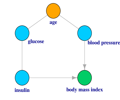
We analyze a real data set originally from the National Institute of Diabetes and Digestive and Kidney Diseases (Smith et al., 1988). The dataset consists of serval medical predictor variables for the outcome of diabetes. We are interested in the causal structural of five variables: age, body mass index, 2-hour serum insulin, plasma glucose concentration and diastolic blood pressure. After removing the missing data, we obtain n=392n=392 samples. The PC–algorithm is applied to examine the causal structure of the five variables based on the four different conditional independence measures. We implement the causal algorithms by the R package pcalg (Kalisch et al., 2012). The estimated causal structure are shown in Figure 2. The proposed test gives the same estimated graph as the partial correlation, since the data is approximately normally distributed. To interpret the graph, note that age is likely to affect the diastolic blood pressure. The plasma glucose concentration level is also likely to be related to age. This is confirmed by the causal findings of (a), (b) and (c) in Figure 2. Besides, serum insulin has plausible causal effects on body mass index, and is also related to plasma glucose concentration. The causal relationship between age and blood pressure is not confirmed in part (c), the test of conditional mutual information. This is not a surprise given the high false positive rate reported in Table 5 in the appendix. The kernel based conditional independence is a little conservative and is not able to detect some of the possible edges. To further illustrate the robustness of the proposed test, we make a logarithm transformation on the data, and apply the same procedure again. The estimated causal structures are reported in Figure 3. We observe that the proposed test results in the same estimated structure as the original data, which echos property (4) in Theorem 1, i.e., the proposed test is invariant with respect to monotone transformations. However, the partial correlation test yields more false positives, since the normality assumption is violated.

Refer to caption Refer to caption (a) (b) Refer to caption Refer to caption (c) (d)

Figure 2: The estimated causal structure of the five variables by using the proposed test in (a), partial correlation in (b), conditional mutual information in (c) and kernel based conditional independence test in (d).

Refer to caption Refer to caption (a) (b) Refer to caption Refer to caption (c) (d)

Figure 3: The estimated causal structure of the log-transformed five variables by using the four tests. Refer to the caption of Figure 2 for the four tests.

5 Discussions

In this paper we developed a new index to measure conditional dependence of random variables and vectors. The calculation of the estimated index requires low computational cost. The test of conditional independence based on the newly proposed index has nontrivial power against all fixed and local alternatives. The proposed test is distribution free under the null hypothesis, and is robust to outliers and heavy-tailed data. Numerical simulations indicate that the proposed test is more powerful than some existing ones. The proposed test is further applied to directed acyclic graphs for causal discovery and shows superior performance.

6 Technical Proofs

6.1 Proof of Proposition 1

For 0<u<10<u<1, define quantile function for XZX\mid Z as

FXZ1(uZ=z)=inf{x:FXZ(xZ=z)u}.F_{X\mid Z}^{-1}(u\mid Z=z)=\inf\{x:F_{X\mid Z}(x\mid Z=z)\geq u\}.

Similarly, we can define FYZ1(vZ=z)F_{Y\mid Z}^{-1}(v\mid Z=z), the quantile function for YZY\mid Z, for 0<v<10<v<1. Since XX and YY have continuous conditional distribution functions for every given value of ZZ, it follows that when 0<u<10<u<1 and 0<v<10<v<1,

Pr{FXZ(XZ)u,FYZ(YZ)vZ=z}\displaystyle\mbox{Pr}\{F_{X\mid Z}(X\mid Z)\leq u,F_{Y\mid Z}(Y\mid Z)\leq v\mid Z=z\}
=\displaystyle= Pr{XFXZ1(uZ),YFYZ1(vZ)Z=z}.\displaystyle\mbox{Pr}\{X\leq F_{X\mid Z}^{-1}(u\mid Z),Y\leq F_{Y\mid Z}^{-1}(v\mid Z)\mid Z=z\}.

This implies that XYZX\bot\!\!\!\bot Y\mid Z is equivalent to UVZU\bot\!\!\!\bot V\mid Z. In addition, conditional on Z=zZ=z, FXZ(XZ=z)F_{X\mid Z}(X\mid Z=z) is uniformly distributed on (0,1)(0,1), which does not depend on the particular value of zz, indicating FXZ(XZ)ZF_{X\mid Z}(X\mid Z)\bot\!\!\!\bot Z. That is, UZU\bot\!\!\!\bot Z. Similarly, VZV\bot\!\!\!\bot Z. Thus, the conditional independence fU,VZ(u,vz)=fUZ(uz)fVZ(vz)f_{U,V\mid Z}(u,v\mid z)=f_{U\mid Z}(u\mid z)f_{V\mid Z}(v\mid z) together with fUZ(uz)=fU(u)f_{U\mid Z}(u\mid z)=f_{U}(u) and fVZ(vz)=fV(v)f_{V\mid Z}(v\mid z)=f_{V}(v) implies that

fU,VZ(u,vz)=fU(u)fV(v).\displaystyle f_{U,V\mid Z}(u,v\mid z)=f_{U}(u)f_{V}(v).

Thus, UU, VV and ZZ are mutually independent.

On the other hand, the mutual independence immediately leads to the conditional independence UVZU\bot\!\!\!\bot V\mid Z. Therefore, the conditional independence XYZX\bot\!\!\!\bot Y\mid Z is equivalent to the mutual independence of UU, VV and ZZ. We next show that the mutual independence of UU, VV and ZZ is equivalent to mutual independence of UU, VV and WW.

Define FZ1(w)=inf{z:F(z)w}F_{Z}^{-1}(w)=\inf\{z:F(z)\geq w\} for 0<w<10<w<1. If UU, VV and ZZ are mutually independent, then

Pr(Uu,Vv,Ww)=Pr{Uu,Vv,ZFZ1(w)}\displaystyle\mbox{Pr}(U\leq u,V\leq v,W\leq w)=\mbox{Pr}\{U\leq u,V\leq v,Z\leq F_{Z}^{-1}(w)\}
=\displaystyle= Pr(Uu)Pr(Vv)Pr{ZFZ1(w)}=Pr(Uu)Pr(Vv)Pr(Ww)\displaystyle\mbox{Pr}(U\leq u)\mbox{Pr}(V\leq v)\mbox{Pr}\{Z\leq F_{Z}^{-1}(w)\}=\mbox{Pr}(U\leq u)\mbox{Pr}(V\leq v)\mbox{Pr}(W\leq w)

holds for all u,u, vv and ww. On the other hand, if UU, VV and WW are mutually independent, it follows that

Pr(Uu,Vv,Zz)=Pr{Uu,Vv,WFZ(z)}\displaystyle\mbox{Pr}(U\leq u,V\leq v,Z\leq z)=\mbox{Pr}\{U\leq u,V\leq v,W\leq F_{Z}(z)\}
=\displaystyle= Pr(Uu)Pr(Vv)Pr{WFZ(z)}=Pr(Uu)Pr(Vv)Pr(Zz),\displaystyle\mbox{Pr}(U\leq u)\mbox{Pr}(V\leq v)\mbox{Pr}\{W\leq F_{Z}(z)\}=\mbox{Pr}(U\leq u)\mbox{Pr}(V\leq v)\mbox{Pr}(Z\leq z),

holds for all u,u, vv and zz. Thus, the mutual independence of UU, VV and ZZ is equivalent to the mutual independence of UU, VV and WW. This completes the proof.

6.2 Proof of Theorem 1

We start with the derivation of the index ρ\rho. UU, VV and WW are mutually independent if and only if

φU,V,W(t1,t2,t3)φU(t1)φV(t2)φW(t3)2ω(t1,t2,t3)𝑑t1𝑑t2𝑑t3=0,\displaystyle\iiint\left\|\varphi_{U,V,W}(t_{1},t_{2},t_{3})-\varphi_{U}(t_{1})\varphi_{V}(t_{2})\varphi_{W}(t_{3})\right\|^{2}\omega(t_{1},t_{2},t_{3})dt_{1}dt_{2}dt_{3}=0, (5)

for arbitrary positive weight function ω()\omega(\cdot). We now show that the proposed index ρ\rho is proportional to the integration in (5) by choosing ω(t1,t2,t3)\omega(t_{1},t_{2},t_{3}) to be the joint probability density function of three independent and identically distributed standard Cauchy random variables.

With some calculation and Fubini’s theorem, we have

φU,V,W(t1,t2,t3)φU(t1)φV(t2)φW(t3)2ω(t1,t2,t3)𝑑t1𝑑t2𝑑t3\displaystyle\iiint\left\|\varphi_{U,V,W}(t_{1},t_{2},t_{3})-\varphi_{U}(t_{1})\varphi_{V}(t_{2})\varphi_{W}(t_{3})\right\|^{2}\omega(t_{1},t_{2},t_{3})dt_{1}dt_{2}dt_{3}
=\displaystyle= Eeit1(U1U2)+it2(V1V2)+it3(W1W2)ω(t1,t2,t3)𝑑t1𝑑t2𝑑t3\displaystyle E\iiint e^{it_{1}(U_{1}-U_{2})+it_{2}(V_{1}-V_{2})+it_{3}(W_{1}-W_{2})}\omega(t_{1},t_{2},t_{3})dt_{1}dt_{2}dt_{3}
Eeit1(U1U3)+it2(V1V4)+it3(W1W2)ω(t1,t2,t3)𝑑t1𝑑t2𝑑t3\displaystyle-E\iiint e^{it_{1}(U_{1}-U_{3})+it_{2}(V_{1}-V_{4})+it_{3}(W_{1}-W_{2})}\omega(t_{1},t_{2},t_{3})dt_{1}dt_{2}dt_{3}
Eeit1(U3U1)+it2(V4V1)+it3(W2W1)ω(t1,t2,t3)𝑑t1𝑑t2𝑑t3\displaystyle-E\iiint e^{it_{1}(U_{3}-U_{1})+it_{2}(V_{4}-V_{1})+it_{3}(W_{2}-W_{1})}\omega(t_{1},t_{2},t_{3})dt_{1}dt_{2}dt_{3}
+Eeit1(U1U2)+it2(V3V4)+it3(W5W6)ω(t1,t2,t3)𝑑t1𝑑t2𝑑t3.\displaystyle+E\iiint e^{it_{1}(U_{1}-U_{2})+it_{2}(V_{3}-V_{4})+it_{3}(W_{5}-W_{6})}\omega(t_{1},t_{2},t_{3})dt_{1}dt_{2}dt_{3}.

According to the property of characteristic function for standard Cauchy distribution, we have

eit(U1U2)π1(1+t2)1𝑑t=e|U1U2|.\displaystyle\int e^{it(U_{1}-U_{2})}\pi^{-1}(1+t^{2})^{-1}dt=e^{-|U_{1}-U_{2}|}.

Then by choosing ω(t1,t2,t3)=π3(1+t12)1(1+t22)1(1+t32)1\omega(t_{1},t_{2},t_{3})=\pi^{-3}(1+t_{1}^{2})^{-1}(1+t_{2}^{2})^{-1}(1+t_{3}^{2})^{-1}, i.e., the joint density function of three i.i.d. standard Cauchy distributions, we have

φU,V,W(t1,t2,t3)φU(t1)φV(t2)φW(t3)2ω(t1,t2,t3)𝑑t1𝑑t2𝑑t3=Ee|U1U2||V1V2||W1W2|2Ee|U1U3||V1V4||W1W2|+Ee|U1U2|Ee|V1V2|Ee|W1W2|.\displaystyle\begin{split}&\iiint\left\|\varphi_{U,V,W}(t_{1},t_{2},t_{3})-\varphi_{U}(t_{1})\varphi_{V}(t_{2})\varphi_{W}(t_{3})\right\|^{2}\omega(t_{1},t_{2},t_{3})dt_{1}dt_{2}dt_{3}\\ &=Ee^{-|U_{1}-U_{2}|-|V_{1}-V_{2}|-|W_{1}-W_{2}|}-2Ee^{-|U_{1}-U_{3}|-|V_{1}-V_{4}|-|W_{1}-W_{2}|}\\ &\hskip 28.45274pt+Ee^{-|U_{1}-U_{2}|}Ee^{-|V_{1}-V_{2}|}Ee^{-|W_{1}-W_{2}|}.\end{split} (6)

Furthermore, with the fact that UWU\bot\!\!\!\bot W and VWV\bot\!\!\!\bot W, (6) is equal to

E{SU(U1,U2)SV(V1,V2)e|W1W2|},\displaystyle E\left\{S_{U}(U_{1},U_{2})S_{V}(V_{1},V_{2})e^{-|W_{1}-W_{2}|}\right\},

where SU(U1,U2)S_{U}(U_{1},U_{2}) and SV(V1,V2)S_{V}(V_{1},V_{2}) are defined as

SU(U1,U2)\displaystyle S_{U}(U_{1},U_{2}) =\displaystyle= E{e|U1U2|+e|U3U4|e|U1U3|e|U2U3|(U1,U2)},\displaystyle E\left\{e^{-|U_{1}-U_{2}|}+e^{-|U_{3}-U_{4}|}-e^{-|U_{1}-U_{3}|}-e^{-|U_{2}-U_{3}|}\mid(U_{1},U_{2})\right\},
SV(V1,V2)\displaystyle S_{V}(V_{1},V_{2}) =\displaystyle= E{e|V1V2|+e|V3V4|e|V1V3|e|V2V3|(V1,V2)}.\displaystyle E\left\{e^{-|V_{1}-V_{2}|}+e^{-|V_{3}-V_{4}|}-e^{-|V_{1}-V_{3}|}-e^{-|V_{2}-V_{3}|}\mid(V_{1},V_{2})\right\}.

Now we calculate the normalization constant c0c_{0}. It follows by the Cauchy-Schwarz inequality that

E{SU(U1,U2)SV(V1,V2)e|W1W2|}\displaystyle E\left\{S_{U}(U_{1},U_{2})S_{V}(V_{1},V_{2})e^{-|W_{1}-W_{2}|}\right\}
=\displaystyle= E[e|W1W2|E{SU(U1,U2)SV(V1,V2)(W1,W2)}]\displaystyle E\left[e^{-|W_{1}-W_{2}|}E\left\{S_{U}(U_{1},U_{2})S_{V}(V_{1},V_{2})\mid(W_{1},W_{2})\right\}\right]
\displaystyle\leq E[e|W1W2|E1/2{SU2(U1,U2)(W1,W2)}E1/2{SV2(V1,V2)(W1,W2)}]\displaystyle E\left[e^{-|W_{1}-W_{2}|}E^{1/2}\left\{S_{U}^{2}(U_{1},U_{2})\mid(W_{1},W_{2})\right\}E^{1/2}\left\{S_{V}^{2}(V_{1},V_{2})\mid(W_{1},W_{2})\right\}\right]
=\displaystyle= E[e|W1W2|E1/2{SU2(U1,U2)}E1/2{SV2(V1,V2)}]\displaystyle E\left[e^{-|W_{1}-W_{2}|}E^{1/2}\left\{S_{U}^{2}(U_{1},U_{2})\right\}E^{1/2}\left\{S_{V}^{2}(V_{1},V_{2})\right\}\right]
=\displaystyle= 2e1(6.5e220e1+6.5)\displaystyle 2e^{-1}(6.5e^{-2}-20e^{-1}+6.5)
=def\displaystyle\stackrel{{\scriptstyle\mbox{{\rm\tiny def}}}}{{=}} c01,\displaystyle c_{0}^{-1},

where the equality holds if and only if SU(U1,U2)=λ{SV(V1,V2)}S_{U}(U_{1},U_{2})=\lambda\left\{S_{V}(V_{1},V_{2})\right\} holds with probability 1, where λ0\lambda\geq 0 (because E{SU(U1,U2)SV(V1,V2)}E\left\{S_{U}(U_{1},U_{2})S_{V}(V_{1},V_{2})\right\} is nonnegative). Recall that UU, VV and WW are all uniformly distributed on (0,1)(0,1), further calculations give us

SU(U1,U2)\displaystyle S_{U}(U_{1},U_{2}) =\displaystyle= e|U1U2|+eU1+eU11+eU2+eU21+2e14,\displaystyle e^{-|U_{1}-U_{2}|}+e^{-U_{1}}+e^{U_{1}-1}+e^{-U_{2}}+e^{U_{2}-1}+2e^{-1}-4,
SV(V1,V2)\displaystyle S_{V}(V_{1},V_{2}) =\displaystyle= e|V1V2|+eV1+eV11+eV2+eV21+2e14.\displaystyle e^{-|V_{1}-V_{2}|}+e^{-V_{1}}+e^{V_{1}-1}+e^{-V_{2}}+e^{V_{2}-1}+2e^{-1}-4.

This, together with the normalization constant c0c_{0}, yield the expression of the index ρ(X,YZ)\rho(X,Y\mid Z). Subsequently, the properties of the index ρ(X,YZ)\rho(X,Y\mid Z) can be established.

(1) ρ(X,YZ)0\rho(X,Y\mid Z)\geq 0 holds obviously. It equals 0 only when UU, VV, WW are mutual independent, which is equivalent to the conditional independence XYZX\bot\!\!\!\bot Y\mid Z. ρ(X,YZ)1\rho(X,Y\mid Z)\leq 1 holds obviously according to the derivation of the index ρ\rho. The equality holds if and only if SU(U1,U2)=λ{SV(V1,V2)}S_{U}(U_{1},U_{2})=\lambda\left\{S_{V}(V_{1},V_{2})\right\}. Because ESU2(U1,U2)=ESV2(V1,V2)ES_{U}^{2}(U_{1},U_{2})=ES_{V}^{2}(V_{1},V_{2}), we have λ=1\lambda=1. If U=VU=V or U+V=1U+V=1, it is easy to check SU(U1,U2)=SV(V1,V2)S_{U}(U_{1},U_{2})=S_{V}(V_{1},V_{2}). This completes the proof of Part (1).

(2) This property is trivial according to the definition of ρ\rho.

(3) For strictly monotone transformations m3()m_{3}(\cdot), we have when m1()m_{1}(\cdot) is strictly increasing, Um=Fm1(X)m3(Z){m1(X)m3(Z)}U_{m}=F_{m_{1}(X)\mid m_{3}(Z)}\{m_{1}(X)\mid m_{3}(Z)\} equals U=FXZ(XZ)U=F_{X\mid Z}(X\mid Z), while when m1()m_{1}(\cdot) is strictly decreasing, it equals 1U1-U. It can be easily verified that SU(U1,U2)=SU(1U1,1U2)S_{U}(U_{1},U_{2})=S_{U}(1-U_{1},1-U_{2}), then we have SUm(Um1,Um2)=SU(U1,U2)S_{U_{m}}(U_{m1},U_{m2})=S_{U}(U_{1},U_{2}) no matter whether m1()m_{1}(\cdot) is strictly increasing or decreasing. Similarly, let Vm=Fm2(Y)m3(Z){m2(Y)m3(Z)}V_{m}=F_{m_{2}(Y)\mid m_{3}(Z)}\{m_{2}(Y)\mid m_{3}(Z)\}, we obtain that SVm(Vm1,Vm2)=SV(V1,V2)S_{V_{m}}(V_{m1},V_{m2})=S_{V}(V_{1},V_{2}). It is clear that Wm=Fm3(Z){m3(Z)}W_{m}=F_{m_{3}(Z)}\{m_{3}(Z)\} equals either WW or 1W1-W, implying e|Wm1Wm2|=e|W1W2|e^{-|W_{m1}-W_{m2}|}=e^{-|W_{1}-W_{2}|}. Therefore, we have

E{SUm(Um1,Um2)SVm(Vm1,Vm2)e|Wm1Wm2|}=E{SU(U1,U2)SV(V1,V2)e|W1W2|},\displaystyle E\left\{S_{U_{m}}(U_{m1},U_{m2})S_{V_{m}}(V_{m1},V_{m2})e^{-|W_{m1}-W_{m2}|}\right\}=E\left\{S_{U}(U_{1},U_{2})S_{V}(V_{1},V_{2})e^{-|W_{1}-W_{2}|}\right\},

and it is true that ρ{m1(X),m2(Y)m3(Z)}=ρ(X,YZ)\rho\left\{m_{1}(X),m_{2}(Y)\mid m_{3}(Z)\right\}=\rho(X,Y\mid Z).

6.3 Proof of Theorem 2

For simplicity, we denote by g(x)=e|x|g(x)=e^{-|x|} and S0(x,y)=g(xy)+ex+ex1+ey+ey1+2e14S_{0}(x,y)=g\left(x-y\right)+e^{-x}+e^{x-1}+e^{-y}+e^{y-1}+2e^{-1}-4. We write c01ρ^(X,YZ)c_{0}^{-1}\widehat{\rho}(X,Y\mid Z) as

n2i,j{S0(U^i,U^j)S0(V^i,V^j)g(W^iW^j)}.\displaystyle n^{-2}\sum_{i,j}\left\{S_{0}(\widehat{U}_{i},\widehat{U}_{j})S_{0}(\widehat{V}_{i},\widehat{V}_{j})g(\widehat{W}_{i}-\widehat{W}_{j})\right\}.

With Taylor’s expansion, when nh4m0nh^{4m}\to 0 and nh2/log2(n)nh^{2}/\log^{2}(n)\to\infty, we have

S0(U^i,U^j)\displaystyle S_{0}(\widehat{U}_{i},\widehat{U}_{j})
=\displaystyle= {g(UiUj)+eUi1eUi}ΔUi{g(UiUj)eUj1+eUj}ΔUj\displaystyle\left\{g^{\prime}\left(U_{i}-U_{j}\right)+e^{U_{i}-1}-e^{-U_{i}}\right\}\Delta U_{i}-\left\{g^{\prime}\left(U_{i}-U_{j}\right)-e^{U_{j}-1}+e^{-U_{j}}\right\}\Delta U_{j}
+\displaystyle+ 21{g′′(UiUj)(ΔUiΔUj)2+(eUi+eUi1)(ΔUi)2+(eUj+eUj1)(ΔUj)2}\displaystyle 2^{-1}\left\{g^{\prime\prime}\left(U_{i}-U_{j}\right)(\Delta U_{i}-\Delta U_{j})^{2}+\left(e^{-U_{i}}+e^{U_{i}-1}\right)(\Delta U_{i})^{2}+\left(e^{-U_{j}}+e^{U_{j}-1}\right)(\Delta U_{j})^{2}\right\}
+\displaystyle+ 61{g′′′(UiUj)(ΔUiΔUj)3+(eUi1eUi)(ΔUi)3+(eUj1eUj)(ΔUj)3}\displaystyle 6^{-1}\left\{g^{\prime\prime\prime}\left(U_{i}-U_{j}\right)(\Delta U_{i}-\Delta U_{j})^{3}+\left(e^{U_{i}-1}-e^{-U_{i}}\right)(\Delta U_{i})^{3}+\left(e^{U_{j}-1}-e^{-U_{j}}\right)(\Delta U_{j})^{3}\right\}
+\displaystyle+ S0(Ui,Uj)+op(n1)\displaystyle S_{0}\left(U_{i},U_{j}\right)+o_{p}(n^{-1})
=def\displaystyle\stackrel{{\scriptstyle\mbox{{\rm\tiny def}}}}{{=}} S1(Ui,Uj)+S2(Ui,Uj)+S3(Ui,Uj)+S0(Ui,Uj)+op(n1),\displaystyle S_{1}(U_{i},U_{j})+S_{2}(U_{i},U_{j})+S_{3}(U_{i},U_{j})+S_{0}(U_{i},U_{j})+o_{p}(n^{-1}),

where ΔUi=U^iUi\Delta U_{i}=\widehat{U}_{i}-U_{i}, and Sk(Ui,Uj),k=1,2,3S_{k}(U_{i},U_{j}),k=1,2,3 are defined to be each row in an obvious way. Similarly, we expand S0(V^i,V^j)S_{0}(\widehat{V}_{i},\widehat{V}_{j}) as

S0(V^i,V^j)\displaystyle S_{0}(\widehat{V}_{i},\widehat{V}_{j}) =\displaystyle= S0(Vi,Vj)+S1(Vi,Vj)+S2(Vi,Vj)+S3(Vi,Vj)+op(n1).\displaystyle S_{0}(V_{i},V_{j})+S_{1}(V_{i},V_{j})+S_{2}(V_{i},V_{j})+S_{3}(V_{i},V_{j})+o_{p}(n^{-1}).

As for g(W^iW^j)g(\widehat{W}_{i}-\widehat{W}_{j}), we have

g(W^iW^j)\displaystyle g(\widehat{W}_{i}-\widehat{W}_{j}) =\displaystyle= g(WiWj)+g(WiWj)(ΔWiΔWj)\displaystyle g(W_{i}-W_{j})+g^{\prime}(W_{i}-W_{j})(\Delta W_{i}-\Delta W_{j})
+21g′′(WiWj)(ΔWiΔWj)2+op(n1).\displaystyle+2^{-1}g^{\prime\prime}(W_{i}-W_{j})(\Delta W_{i}-\Delta W_{j})^{2}+o_{p}(n^{-1}).

Therefore, it follows that

c01ρ^(X,YZ)\displaystyle c_{0}^{-1}\widehat{\rho}(X,Y\mid Z) =\displaystyle= 21n2i,jS0(Ui,Uj)S0(Vi,Vj)g′′(WiWj)(ΔWiΔWj)2\displaystyle 2^{-1}n^{-2}\sum_{i,j}S_{0}\left(U_{i},U_{j}\right)S_{0}\left(V_{i},V_{j}\right)g^{\prime\prime}(W_{i}-W_{j})(\Delta W_{i}-\Delta W_{j})^{2}
+n2i,j0k+l1Sk(Ui,Uj)Sl(Vi,Vj)g(WiWj)(ΔWiΔWj)\displaystyle+n^{-2}\sum_{i,j}\sum_{0\leq k+l\leq 1}S_{k}\left(U_{i},U_{j}\right)S_{l}\left(V_{i},V_{j}\right)g^{\prime}(W_{i}-W_{j})(\Delta W_{i}-\Delta W_{j})
+n2i,j0k+l3Sk(Ui,Uj)Sl(Vi,Vj)g(WiWj)+op(n1)\displaystyle+n^{-2}\sum_{i,j}\sum_{0\leq k+l\leq 3}S_{k}\left(U_{i},U_{j}\right)S_{l}\left(V_{i},V_{j}\right)g\left(W_{i}-W_{j}\right)+o_{p}(n^{-1})
=def\displaystyle\stackrel{{\scriptstyle\mbox{{\rm\tiny def}}}}{{=}} 21Q1+Q2+Q3+op(n1).\displaystyle 2^{-1}Q_{1}+Q_{2}+Q_{3}+o_{p}(n^{-1}).

We first show that Q1Q_{1} is of order op(n1)o_{p}(n^{-1}). In fact,

Q1\displaystyle Q_{1} =\displaystyle= n2i,jS0(Ui,Uj)S0(Vi,Vj)g′′(WiWj)(ΔWiΔWj)2\displaystyle n^{-2}\sum_{i,j}S_{0}\left(U_{i},U_{j}\right)S_{0}\left(V_{i},V_{j}\right)g^{\prime\prime}(W_{i}-W_{j})(\Delta W_{i}-\Delta W_{j})^{2}
=\displaystyle= n2i,jS0(Ui,Uj)S0(Vi,Vj)g′′(WiWj){(ΔWi)2+(ΔWj)2}\displaystyle n^{-2}\sum_{i,j}S_{0}\left(U_{i},U_{j}\right)S_{0}\left(V_{i},V_{j}\right)g^{\prime\prime}(W_{i}-W_{j})\left\{\left(\Delta W_{i}\right)^{2}+\left(\Delta W_{j}\right)^{2}\right\}
+2n2i,jS0(Ui,Uj)S0(Vi,Vj)g′′(WiWj)(WiΔWj+WjΔWi)\displaystyle+2n^{-2}\sum_{i,j}S_{0}\left(U_{i},U_{j}\right)S_{0}\left(V_{i},V_{j}\right)g^{\prime\prime}(W_{i}-W_{j})(W_{i}\Delta W_{j}+W_{j}\Delta W_{i})
2n2i,jS0(Ui,Uj)S0(Vi,Vj)g′′(WiWj)(W^iW^jWiWj)\displaystyle-2n^{-2}\sum_{i,j}S_{0}\left(U_{i},U_{j}\right)S_{0}\left(V_{i},V_{j}\right)g^{\prime\prime}(W_{i}-W_{j})(\widehat{W}_{i}\widehat{W}_{j}-W_{i}W_{j})
=def\displaystyle\stackrel{{\scriptstyle\mbox{{\rm\tiny def}}}}{{=}} Q1,1+Q1,2+Q1,3.\displaystyle Q_{1,1}+Q_{1,2}+Q_{1,3}.

Under the null hypothesis, UU, VV and WW are mutually independent, it is easy to verify that E{S0(Ui,Uj)(Ui,Vi,Wi,Vj,Wj)}=0E\left\{S_{0}\left(U_{i},U_{j}\right)\mid(U_{i},V_{i},W_{i},V_{j},W_{j})\right\}=0, and hence

E{S0(Ui,Uj)S0(Vi,Vj)g′′(WiWj)(Ui,Vi,Wi)}=0.\displaystyle E\left\{S_{0}\left(U_{i},U_{j}\right)S_{0}\left(V_{i},V_{j}\right)g^{\prime\prime}(W_{i}-W_{j})\mid(U_{i},V_{i},W_{i})\right\}=0.

Then for each fixed ii, we have

n1jS0(Ui,Uj)S0(Vi,Vj)g′′(WiWj)=Op(n1/2).\displaystyle n^{-1}\sum_{j}S_{0}\left(U_{i},U_{j}\right)S_{0}\left(V_{i},V_{j}\right)g^{\prime\prime}(W_{i}-W_{j})=O_{p}(n^{-1/2}).

Thus, Q1,1Q_{1,1} is clearly of order op(n1)o_{p}(n^{-1}) because (ΔWi)2=op(n1/2)\left(\Delta W_{i}\right)^{2}=o_{p}(n^{-1/2}). Now we deal with Q1,2Q_{1,2}.

n2i,jS0(Ui,Uj)S0(Vi,Vj)g′′(WiWj)WiΔWj\displaystyle n^{-2}\sum_{i,j}S_{0}\left(U_{i},U_{j}\right)S_{0}\left(V_{i},V_{j}\right)g^{\prime\prime}(W_{i}-W_{j})W_{i}\Delta W_{j}
=n3i,j,kS0(Ui,Uj)S0(Vi,Vj)g′′(WiWj)Wi{𝟙(WkWj)Wj}.\displaystyle=n^{-3}\sum_{i,j,k}S_{0}\left(U_{i},U_{j}\right)S_{0}\left(V_{i},V_{j}\right)g^{\prime\prime}(W_{i}-W_{j})W_{i}\left\{\mathbbm{1}(W_{k}\leq W_{j})-W_{j}\right\}.

Under the null hypothesis, because E{S0(Ui,Uj)(Ui,Vi,Wi,Vj,Wj)}=0E\left\{S_{0}\left(U_{i},U_{j}\right)\mid(U_{i},V_{i},W_{i},V_{j},W_{j})\right\}=0, WW is uniformly distributed, we have E{𝟙(WkWj)Wj}=WjE\{\mathbbm{1}(W_{k}\leq W_{j})\mid W_{j}\}=W_{j}. Thus, the corresponding U-statistic of the equation above is second order degenerate. In addition, when any two of i,j,ki,j,k are identical, we have

E[S0(Ui,Uj)S0(Vi,Vj)g′′(WiWj)Wi{𝟙(WkWj)Wj}]=0.\displaystyle E\left[S_{0}\left(U_{i},U_{j}\right)S_{0}\left(V_{i},V_{j}\right)g^{\prime\prime}(W_{i}-W_{j})W_{i}\left\{\mathbbm{1}(W_{k}\leq W_{j})-W_{j}\right\}\right]=0.

Then the summations associated with any two of the i,j,ki,j,k are identical is of order op(1)o_{p}(1). Therefore, Q1,2=op(n1)Q_{1,2}=o_{p}(n^{-1}). It remains to deal with Q1,3Q_{1,3}. Similarly, the corresponding U-statistic of

n4i,j,k,lS0(Ui,Uj)S0(Vi,Vj)g′′(WiWj){𝟙(WkWi)𝟙(WlWj)WiWj}\displaystyle n^{-4}\sum_{i,j,k,l}S_{0}\left(U_{i},U_{j}\right)S_{0}\left(V_{i},V_{j}\right)g^{\prime\prime}(W_{i}-W_{j})\left\{\mathbbm{1}(W_{k}\leq W_{i})\mathbbm{1}(W_{l}\leq W_{j})-W_{i}W_{j}\right\}

is second order degenerate and hence we obtain that Q1,3=op(n1)Q_{1,3}=o_{p}(n^{-1}).

Next, we show Q2=op(n1)Q_{2}=o_{p}(n^{-1}). Recall that

Q2\displaystyle Q_{2} =\displaystyle= n2i,jS0(Ui,Uj)S0(Vi,Vj)g(WiWj)(ΔWiΔWj)\displaystyle n^{-2}\sum_{i,j}S_{0}\left(U_{i},U_{j}\right)S_{0}\left(V_{i},V_{j}\right)g^{\prime}(W_{i}-W_{j})(\Delta W_{i}-\Delta W_{j})
+2n2i,jS1(Ui,Uj)S0(Vi,Vj)g(WiWj)ΔWi\displaystyle+2n^{-2}\sum_{i,j}S_{1}\left(U_{i},U_{j}\right)S_{0}\left(V_{i},V_{j}\right)g^{\prime}(W_{i}-W_{j})\Delta W_{i}
+2n2i,jS0(Ui,Uj)S1(Vi,Vj)g(WiWj)ΔWi\displaystyle+2n^{-2}\sum_{i,j}S_{0}\left(U_{i},U_{j}\right)S_{1}\left(V_{i},V_{j}\right)g^{\prime}(W_{i}-W_{j})\Delta W_{i}
=def\displaystyle\stackrel{{\scriptstyle\mbox{{\rm\tiny def}}}}{{=}} Q2,1+2Q2,2+2Q2,3.\displaystyle Q_{2,1}+2Q_{2,2}+2Q_{2,3}.

Similar to dealing with Q1,2Q_{1,2}, we have Q2,1=op(n1)Q_{2,1}=o_{p}(n^{-1}). We now evaluate Q2,2Q_{2,2}.

Q2,2\displaystyle Q_{2,2} =\displaystyle= n2i,j{g(UiUj)+eUi1eUi}ΔUiS0(Vi,Vj)g(WiWj)ΔWi\displaystyle n^{-2}\sum_{i,j}\left\{g^{\prime}\left(U_{i}-U_{j}\right)+e^{U_{i}-1}-e^{-U_{i}}\right\}\Delta U_{i}S_{0}\left(V_{i},V_{j}\right)g^{\prime}(W_{i}-W_{j})\Delta W_{i}
n2i,j{g(UiUj)eUj1+eUj}ΔUjS0(Vi,Vj)g(WiWj)ΔWi.\displaystyle-n^{-2}\sum_{i,j}\left\{g^{\prime}\left(U_{i}-U_{j}\right)-e^{U_{j}-1}+e^{-U_{j}}\right\}\Delta U_{j}S_{0}\left(V_{i},V_{j}\right)g^{\prime}(W_{i}-W_{j})\Delta W_{i}.

Because under the null hypothesis, E{S0(Vi,Vj)(Ui,Vi,Wi,Uj,Wj)}=0E\left\{S_{0}\left(V_{i},V_{j}\right)\mid(U_{i},V_{i},W_{i},U_{j},W_{j})\right\}=0, it follows that for each ii,

n1j{g(UiUj)+eUi1eUi}S0(Vi,Vj)g(WiWj)=Op(n1/2),\displaystyle n^{-1}\sum_{j}\left\{g^{\prime}\left(U_{i}-U_{j}\right)+e^{U_{i}-1}-e^{-U_{i}}\right\}S_{0}\left(V_{i},V_{j}\right)g^{\prime}(W_{i}-W_{j})=O_{p}(n^{-1/2}),

and the first term of Q2,2Q_{2,2} is of order op(n1)o_{p}(n^{-1}) because ΔWi=Op(n1/2)\Delta W_{i}=O_{p}(n^{-1/2}) and ΔUi=op(1)\Delta U_{i}=o_{p}(1). In addition, for each jj,

n2i,k{g(UiUj)eUj1+eUj}S0(Vi,Vj)g(WiWj){𝟙(WkWi)Wi}\displaystyle n^{-2}\sum_{i,k}\left\{g^{\prime}\left(U_{i}-U_{j}\right)-e^{U_{j}-1}+e^{-U_{j}}\right\}S_{0}\left(V_{i},V_{j}\right)g^{\prime}(W_{i}-W_{j})\left\{\mathbbm{1}(W_{k}\leq W_{i})-W_{i}\right\}

is degenerate and hence the second term of Q2,2Q_{2,2} is also of order op(n1)o_{p}(n^{-1}) because ΔUj=op(1)\Delta U_{j}=o_{p}(1), indicating Q2,2=op(n1)Q_{2,2}=o_{p}(n^{-1}). Similarly, we have Q2,3=op(n1)Q_{2,3}=o_{p}(n^{-1}). Thus it follows that Q2=op(n1)Q_{2}=o_{p}(n^{-1}).

Finally, we show that Q3=n2i,jS0(Ui,Uj)S0(Vi,Vj)g(WiWj)+op(n1)Q_{3}=n^{-2}\sum_{i,j}S_{0}\left(U_{i},U_{j}\right)S_{0}\left(V_{i},V_{j}\right)g\left(W_{i}-W_{j}\right)+o_{p}(n^{-1}). Or equivalently, we show that Q3,1,Q3,2Q_{3,1},Q_{3,2} and Q3,3Q_{3,3} are all of order op(n1)o_{p}(n^{-1}), where

Q3,1\displaystyle Q_{3,1} =def\displaystyle\stackrel{{\scriptstyle\mbox{{\rm\tiny def}}}}{{=}} n2i,jk+l=1Sk(Ui,Uj)Sl(Vi,Vj)g(WiWj),\displaystyle n^{-2}\sum_{i,j}\sum_{k+l=1}S_{k}\left(U_{i},U_{j}\right)S_{l}\left(V_{i},V_{j}\right)g\left(W_{i}-W_{j}\right),
Q3,2\displaystyle Q_{3,2} =def\displaystyle\stackrel{{\scriptstyle\mbox{{\rm\tiny def}}}}{{=}} n2i,jk+l=2Sk(Ui,Uj)Sl(Vi,Vj)g(WiWj),\displaystyle n^{-2}\sum_{i,j}\sum_{k+l=2}S_{k}\left(U_{i},U_{j}\right)S_{l}\left(V_{i},V_{j}\right)g\left(W_{i}-W_{j}\right),
Q3,3\displaystyle Q_{3,3} =def\displaystyle\stackrel{{\scriptstyle\mbox{{\rm\tiny def}}}}{{=}} n2i,jk+l=3Sk(Ui,Uj)Sl(Vi,Vj)g(WiWj).\displaystyle n^{-2}\sum_{i,j}\sum_{k+l=3}S_{k}\left(U_{i},U_{j}\right)S_{l}\left(V_{i},V_{j}\right)g\left(W_{i}-W_{j}\right).

We first show that Q3,1=defQ3,1,1+Q3,1,2=op(n1)Q_{3,1}\stackrel{{\scriptstyle\mbox{{\rm\tiny def}}}}{{=}}Q_{3,1,1}+Q_{3,1,2}=o_{p}(n^{-1}), where

Q3,1,1\displaystyle Q_{3,1,1} =\displaystyle= n2i,jS1(Ui,Uj)S0(Vi,Vj)g(WiWj),\displaystyle n^{-2}\sum_{i,j}S_{1}\left(U_{i},U_{j}\right)S_{0}\left(V_{i},V_{j}\right)g\left(W_{i}-W_{j}\right),
Q3,1,2\displaystyle Q_{3,1,2} =\displaystyle= n2i,jS0(Ui,Uj)S1(Vi,Vj)g(WiWj).\displaystyle n^{-2}\sum_{i,j}S_{0}\left(U_{i},U_{j}\right)S_{1}\left(V_{i},V_{j}\right)g\left(W_{i}-W_{j}\right).

Without loss of generality, we only show that Q3,1,1=op(n1)Q_{3,1,1}=o_{p}(n^{-1}). Calculate

S1(Ui,Uj)\displaystyle S_{1}\left(U_{i},U_{j}\right) =\displaystyle= {g(UiUj)+eUi1eUi}ΔUi{g(UiUj)eUj1+eUj}ΔUj,\displaystyle\left\{g^{\prime}\left(U_{i}-U_{j}\right)+e^{U_{i}-1}-e^{-U_{i}}\right\}\Delta U_{i}-\left\{g^{\prime}\left(U_{i}-U_{j}\right)-e^{U_{j}-1}+e^{-U_{j}}\right\}\Delta U_{j},
ΔUi\displaystyle\Delta U_{i} =\displaystyle= n1k=1n[Kh(ZkZi)𝟙(XkXi)f(Zi)UiUi{Kh(ZkZi)f(Zi)}f(Zi)]\displaystyle n^{-1}\sum_{k=1}^{n}\left[\frac{K_{h}(Z_{k}-Z_{i})\mathbbm{1}(X_{k}\leq X_{i})}{f(Z_{i})}-U_{i}-\frac{U_{i}\left\{K_{h}(Z_{k}-Z_{i})-f(Z_{i})\right\}}{f(Z_{i})}\right]
+Op(h2m+n1h1log2n).\displaystyle\hskip 56.9055pt+O_{p}(h^{2m}+n^{-1}h^{-1}\log^{2}n).

Thus, when nh4m0nh^{4m}\to 0 and nh2/log2(n)nh^{2}/\log^{2}(n)\to\infty,

Q3,1,1\displaystyle Q_{3,1,1} =\displaystyle= 2n2i,j{g(UiUj)+eUi1eUi}S0(Vi,Vj)g(WiWj)ΔUi\displaystyle 2n^{-2}\sum_{i,j}\left\{g^{\prime}\left(U_{i}-U_{j}\right)+e^{U_{i}-1}-e^{-U_{i}}\right\}S_{0}\left(V_{i},V_{j}\right)g\left(W_{i}-W_{j}\right)\Delta U_{i}
=\displaystyle= 2n3i,j,k({g(UiUj)+eUi1eUi}S0(Vi,Vj)g(WiWj)\displaystyle 2n^{-3}\sum_{i,j,k}\bigg{(}\left\{g^{\prime}\left(U_{i}-U_{j}\right)+e^{U_{i}-1}-e^{-U_{i}}\right\}S_{0}\left(V_{i},V_{j}\right)g\left(W_{i}-W_{j}\right)
[Kh(ZkZi)𝟙(XkXi)f(Zi)UiUi{Kh(ZkZi)f(Zi)}f(Zi)])+op(n1)\displaystyle\cdot\left[\frac{K_{h}(Z_{k}-Z_{i})\mathbbm{1}(X_{k}\leq X_{i})}{f(Z_{i})}-U_{i}-\frac{U_{i}\left\{K_{h}(Z_{k}-Z_{i})-f(Z_{i})\right\}}{f(Z_{i})}\right]\bigg{)}+o_{p}(n^{-1})
=\displaystyle= 2n(n1)ij({g(UiUj)+eUi1eUi}S0(Vi,Vj)g(WiWj)\displaystyle\frac{2}{n(n-1)}\sum_{i\neq j}\bigg{(}\left\{g^{\prime}\left(U_{i}-U_{j}\right)+e^{U_{i}-1}-e^{-U_{i}}\right\}S_{0}\left(V_{i},V_{j}\right)g\left(W_{i}-W_{j}\right)
[E{Kh(ZkZi)𝟙(XkXi)UiKh(ZkZi)(Xi,Zi)}f(Zi)])+op(n1),\displaystyle\cdot\left[\frac{E\left\{K_{h}(Z_{k}-Z_{i})\mathbbm{1}(X_{k}\leq X_{i})-U_{i}K_{h}(Z_{k}-Z_{i})\mid(X_{i},Z_{i})\right\}}{f(Z_{i})}\right]\bigg{)}+o_{p}(n^{-1}),

where the last equality holds due to equations (2)-(3) of section 5.3.4 in Serfling (2009) and the fact that var{Kh(ZiZj)}=O(h1)\mbox{\rm var}\{K_{h}(Z_{i}-Z_{j})\}=O(h^{-1}). Therefore, since

supXi,Zi|E{Kh(ZkZi)𝟙(XkXi)UiKh(ZkZi)(Xi,Zi)}|=O(hm),\displaystyle\sup_{X_{i},Z_{i}}\big{|}E\left\{K_{h}(Z_{k}-Z_{i})\mathbbm{1}(X_{k}\leq X_{i})-U_{i}K_{h}(Z_{k}-Z_{i})\mid(X_{i},Z_{i})\right\}\big{|}=O(h^{m}),

when the (m1)(m-1)th derivatives of FXZ(xz)fZ(z)F_{X\mid Z}(x\mid z)f_{Z}(z) and fZ(z)f_{Z}(z) with respect to zz are locally Lipschitz-continuous, Q3,1,1Q_{3,1,1} is clearly of order op(n1)o_{p}(n^{-1}) by noting that the summation in the last display is degenerate.

Next, we consider Q3,2Q_{3,2}, where

Q3,2\displaystyle Q_{3,2} =\displaystyle= n2i,jS1(Ui,Uj)S1(Vi,Vj)g(WiWj)\displaystyle n^{-2}\sum_{i,j}S_{1}\left(U_{i},U_{j}\right)S_{1}\left(V_{i},V_{j}\right)g\left(W_{i}-W_{j}\right)
+\displaystyle+ n2i,jS2(Ui,Uj)S0(Vi,Vj)g(WiWj)\displaystyle n^{-2}\sum_{i,j}S_{2}\left(U_{i},U_{j}\right)S_{0}\left(V_{i},V_{j}\right)g\left(W_{i}-W_{j}\right)
+\displaystyle+ n2i,jS0(Ui,Uj)S2(Vi,Vj)g(WiWj)\displaystyle n^{-2}\sum_{i,j}S_{0}\left(U_{i},U_{j}\right)S_{2}\left(V_{i},V_{j}\right)g\left(W_{i}-W_{j}\right)
=def\displaystyle\stackrel{{\scriptstyle\mbox{{\rm\tiny def}}}}{{=}} Q3,2,1+Q3,2,2+Q3,2,3.\displaystyle Q_{3,2,1}+Q_{3,2,2}+Q_{3,2,3}.

We first show that Q3,2,1=op(n1)Q_{3,2,1}=o_{p}(n^{-1}). It follows that

Q3,2,1\displaystyle Q_{3,2,1} =\displaystyle= 2n2i,j[{g(UiUj)+eUi1eUi}{g(ViVj)+eVi1eVi}\displaystyle 2n^{-2}\sum_{i,j}\bigg{[}\left\{g^{\prime}\left(U_{i}-U_{j}\right)+e^{U_{i}-1}-e^{-U_{i}}\right\}\left\{g^{\prime}\left(V_{i}-V_{j}\right)+e^{V_{i}-1}-e^{-V_{i}}\right\}
g(WiWj)ΔUiΔVi]+2n2i,j[{g(UiUj)+eUi1eUi}\displaystyle\cdot g\left(W_{i}-W_{j}\right)\Delta U_{i}\Delta V_{i}\bigg{]}+2n^{-2}\sum_{i,j}\bigg{[}\left\{g^{\prime}\left(U_{i}-U_{j}\right)+e^{U_{i}-1}-e^{-U_{i}}\right\}
{g(ViVj)eVj1+eVj}g(WiWj)ΔUiΔVj]\displaystyle\cdot\left\{g^{\prime}\left(V_{i}-V_{j}\right)-e^{V_{j}-1}+e^{-V_{j}}\right\}g\left(W_{i}-W_{j}\right)\Delta U_{i}\Delta V_{j}\bigg{]}
=def\displaystyle\stackrel{{\scriptstyle\mbox{{\rm\tiny def}}}}{{=}} Q3,2,1,1+Q3,2,1,2.\displaystyle Q_{3,2,1,1}+Q_{3,2,1,2}.

Because E{g(UiUj)+eUi1eUi(Ui,Vi,Wi,Vj,Wj)}=0E\{g^{\prime}\left(U_{i}-U_{j}\right)+e^{U_{i}-1}-e^{-U_{i}}\mid(U_{i},V_{i},W_{i},V_{j},W_{j})\}=0. For each ii,

n1j=1n[{g(UiUj)+eUi1eUi}{g(ViVj)+eVi1eVi}g(WiWj)]\displaystyle n^{-1}\sum_{j=1}^{n}\bigg{[}\left\{g^{\prime}\left(U_{i}-U_{j}\right)+e^{U_{i}-1}-e^{-U_{i}}\right\}\left\{g^{\prime}\left(V_{i}-V_{j}\right)+e^{V_{i}-1}-e^{-V_{i}}\right\}g\left(W_{i}-W_{j}\right)\bigg{]}

is of order Op(n1/2)O_{p}(n^{-1/2}). Then Q3,2,1,1=op(n1)Q_{3,2,1,1}=o_{p}(n^{-1}) because ΔUiΔVi=op(n1/2)\Delta U_{i}\Delta V_{i}=o_{p}(n^{-1/2}). For Q3,2,1,2Q_{3,2,1,2}, ΔUiΔVj=(UiΔVj+UjΔVi)+(U^iV^jUiVj)-\Delta U_{i}\Delta V_{j}=(U_{i}\Delta V_{j}+U_{j}\Delta V_{i})+(\widehat{U}_{i}\widehat{V}_{j}-U_{i}V_{j}). By expanding the U^i\widehat{U}_{i}, U^j\widehat{U}_{j}, V^i\widehat{V}_{i}, V^j\widehat{V}_{j} in Q3,2,1,2Q_{3,2,1,2} as U statistics and apply the same technique as showing Q3,1,1=op(n1)Q_{3,1,1}=o_{p}(n^{-1}) and Q1,3=op(n1)Q_{1,3}=o_{p}(n^{-1}), it follows immediately that Q3,2,1,2Q_{3,2,1,2} is of order op(n1)o_{p}(n^{-1}). Thus Q3,2,1Q_{3,2,1} is of order op(n1)o_{p}(n^{-1}).

For Q3,2,2Q_{3,2,2} and Q3,2,3Q_{3,2,3}, we only show that Q3,2,2Q_{3,2,2} is of order op(n1)o_{p}({n^{-1}}), for simplicity. Recall that S2(Ui,Uj)S_{2}\left(U_{i},U_{j}\right) is defined as

S2(Ui,Uj)\displaystyle S_{2}\left(U_{i},U_{j}\right) =\displaystyle= 21[g′′(UiUj)(ΔUi)2+g′′(UiUj)(ΔUj)2+(eUi+eUi1)(ΔUi)2\displaystyle 2^{-1}\bigg{[}g^{\prime\prime}\left(U_{i}-U_{j}\right)(\Delta U_{i})^{2}+g^{\prime\prime}\left(U_{i}-U_{j}\right)(\Delta U_{j})^{2}+\left(e^{-U_{i}}+e^{U_{i}-1}\right)(\Delta U_{i})^{2}
+(eUj+eUj1)(ΔUj)22g′′(UiUj)ΔUiΔUj].\displaystyle\hskip 56.9055pt+\left(e^{-U_{j}}+e^{U_{j}-1}\right)(\Delta U_{j})^{2}-2g^{\prime\prime}\left(U_{i}-U_{j}\right)\Delta U_{i}\Delta U_{j}\bigg{]}.

The summations associated with either (ΔUi)2(\Delta U_{i})^{2} or (ΔUj)2(\Delta U_{j})^{2} are of order op(n1)o_{p}(n^{-1}) following similar reasons as showing Q3,2,1,1=op(n1)Q_{3,2,1,1}=o_{p}(n^{-1}), and that associated with ΔUiΔUj\Delta U_{i}\Delta U_{j} are of order op(n1)o_{p}(n^{-1}) similar to dealing with Q3,2,1,2Q_{3,2,1,2}. As a result, Q3,2Q_{3,2} is of order op(n1)o_{p}(n^{-1}).

For Q3,3Q_{3,3}, we have

Q3,3=n2i,jk=14S4k(Ui,Uj)Sk1(Vi,Vj)g(WiWj)=defk=14Q3,3,k.\displaystyle Q_{3,3}=n^{-2}\sum_{i,j}\sum_{k=1}^{4}S_{4-k}\left(U_{i},U_{j}\right)S_{k-1}\left(V_{i},V_{j}\right)g\left(W_{i}-W_{j}\right)\stackrel{{\scriptstyle\mbox{{\rm\tiny def}}}}{{=}}\sum_{k=1}^{4}Q_{3,3,k}.

We only show that Q3,3,1=op(n1)Q_{3,3,1}=o_{p}(n^{-1}) because the other terms are similar. Calculate

6S3(Ui,Uj)\displaystyle 6S_{3}\left(U_{i},U_{j}\right)
=\displaystyle= g′′′(UiUj){(ΔUi)33(ΔUi)2ΔUj+3ΔUi(ΔUj)2(ΔUj)3}\displaystyle g^{\prime\prime\prime}\left(U_{i}-U_{j}\right)\left\{(\Delta U_{i})^{3}-3(\Delta U_{i})^{2}\Delta U_{j}+3\Delta U_{i}(\Delta U_{j})^{2}-(\Delta U_{j})^{3}\right\}
+(eUi1eUi)(ΔUi)3+(eUj1eUj)(ΔUj)3.\displaystyle\hskip 85.35826pt+\left(e^{U_{i}-1}-e^{-U_{i}}\right)(\Delta U_{i})^{3}+\left(e^{U_{j}-1}-e^{-U_{j}}\right)(\Delta U_{j})^{3}.

Then the summations associated with either (ΔUi)3(\Delta U_{i})^{3} or (ΔUj)3(\Delta U_{j})^{3} are of order op(n1)o_{p}(n^{-1}) similar to dealing with Q3,2,1,1Q_{3,2,1,1}, and that associated with ΔUi(ΔUj)2\Delta U_{i}(\Delta U_{j})^{2} or (ΔUi)2ΔUj(\Delta U_{i})^{2}\Delta U_{j} are of order op(n1)o_{p}(n^{-1}) similar to the second term of Q2,2Q_{2,2}.

To sum up, we have shown that

c01ρ^(X,YZ)=n2i,jS0(Ui,Uj)S0(Vi,Vj)g(WiWj)+op(n1),\displaystyle c_{0}^{-1}\widehat{\rho}(X,Y\mid Z)=n^{-2}\sum_{i,j}S_{0}\left(U_{i},U_{j}\right)S_{0}\left(V_{i},V_{j}\right)g\left(W_{i}-W_{j}\right)+o_{p}(n^{-1}),

where the right hand side is essentially a first order degenerate V-statistics. Thus by applying Theorem 6.4.1.B of Serfling (2009),

nρ^(X,YZ)𝑑c0j=1λjχj2(1)\displaystyle n\widehat{\rho}(X,Y\mid Z)\xrightarrow{d}c_{0}\sum_{j=1}^{\infty}\lambda_{j}\chi_{j}^{2}(1)

where χj2(1)\chi_{j}^{2}(1), j=1,2,j=1,2,\dots are independent χ2(1)\chi^{2}(1) random variables, and λj\lambda_{j}, j=1,2,j=1,2,\dots are the corresponding eigenvalues of h(u,v,w;u,v,w)h(u,v,w;u^{\prime},v^{\prime},w^{\prime}). It is worth mentioning that the kernel is positive definite and hence all the λj\lambda_{j}s are positive. Therefore, the proof is completed.

6.4 Proof of Theorem 3

Since we generate {Ui,Vi,Wi}\{U_{i}^{*},V_{i}^{*},W_{i}^{*}\}, i=1,,ni=1,\dots,n independently from uniform distribution, it is quite straightforward that U,VU^{*},V^{*} and WW^{*} are mutually independent. In addition, we can write ρ^\widehat{\rho}^{*} as

ρ^=n2i,jc0S0(Ui,Uj)S0(Vi,Vj)g(WiWj),\displaystyle\widehat{\rho}^{*}=n^{-2}\sum_{i,j}c_{0}S_{0}\left(U_{i}^{*},U_{j}^{*}\right)S_{0}\left(V_{i}^{*},V_{j}^{*}\right)g\left(W_{i}^{*}-W_{j}^{*}\right),

which clearly converges in distribution to c0j=1λ~jχj2(1)c_{0}\sum_{j=1}^{\infty}\widetilde{\lambda}_{j}\chi_{j}^{2}(1), where χj2(1)\chi_{j}^{2}(1), j=1,2,j=1,2,\dots are independent χ2(1)\chi^{2}(1) random variables, and λ~j\widetilde{\lambda}_{j}, j=1,2,j=1,2,\dots are the eigenvalues of h(u,v,w;u,v,w)h(u,v,w;u^{\prime},v^{\prime},w^{\prime}), implying λ~j=λj\widetilde{\lambda}_{j}=\lambda_{j}, for j=1,2,j=1,2,\dots, and hence the proof is completed.

6.5 Proof of Theorem 4

We use the same notation as the proof in Theorem 2. With Taylor’s expansion, when nh4m0nh^{4m}\to 0 and nh2/log2(n)nh^{2}/\log^{2}(n)\to\infty, we have

S0(U^i,U^j)\displaystyle S_{0}(\widehat{U}_{i},\widehat{U}_{j}) =\displaystyle= S0(Ui,Uj)+S1(Ui,Uj)+op(n1/2),\displaystyle S_{0}(U_{i},U_{j})+S_{1}(U_{i},U_{j})+o_{p}(n^{-1/2}),
S0(V^i,V^j)\displaystyle S_{0}(\widehat{V}_{i},\widehat{V}_{j}) =\displaystyle= S0(Vi,Vj)+S1(Vi,Vj)+op(n1/2),\displaystyle S_{0}(V_{i},V_{j})+S_{1}(V_{i},V_{j})+o_{p}(n^{-1/2}),
g(W^iW^j)\displaystyle g(\widehat{W}_{i}-\widehat{W}_{j}) =\displaystyle= g(WiWj)+g(WiWj)(ΔWiΔWj)+op(n1/2).\displaystyle g(W_{i}-W_{j})+g^{\prime}(W_{i}-W_{j})(\Delta W_{i}-\Delta W_{j})+o_{p}(n^{-1/2}).

Therefore, we have

c01ρ^(X,YZ)\displaystyle c_{0}^{-1}\widehat{\rho}(X,Y\mid Z) =\displaystyle= n2i,jS0(Ui,Uj)S0(Vi,Vj)g(WiWj)\displaystyle n^{-2}\sum_{i,j}S_{0}\left(U_{i},U_{j}\right)S_{0}\left(V_{i},V_{j}\right)g\left(W_{i}-W_{j}\right)
+n2i,jS0(Ui,Uj)S0(Vi,Vj)g(WiWj)(ΔWiΔWj)\displaystyle+n^{-2}\sum_{i,j}S_{0}\left(U_{i},U_{j}\right)S_{0}\left(V_{i},V_{j}\right)g^{\prime}(W_{i}-W_{j})(\Delta W_{i}-\Delta W_{j})
+n2i,jS1(Ui,Uj)S0(Vi,Vj)g(WiWj)\displaystyle+n^{-2}\sum_{i,j}S_{1}\left(U_{i},U_{j}\right)S_{0}\left(V_{i},V_{j}\right)g(W_{i}-W_{j})
+n2i,jS0(Ui,Uj)S1(Vi,Vj)g(WiWj)+op(n1/2)\displaystyle+n^{-2}\sum_{i,j}S_{0}\left(U_{i},U_{j}\right)S_{1}\left(V_{i},V_{j}\right)g(W_{i}-W_{j})+o_{p}(n^{-1/2})
=def\displaystyle\stackrel{{\scriptstyle\mbox{{\rm\tiny def}}}}{{=}} P1+P2+P3+P4+op(n1/2).\displaystyle P_{1}+P_{2}+P_{3}+P_{4}+o_{p}(n^{-1/2}).

We deal with the four terms, respectively. For P1P_{1}, by applying Lemma 5.7.3 and equation (2) in section 5.3.1 of Serfling (2009), we have

P1c01ρ(X,YZ)\displaystyle P_{1}-c_{0}^{-1}\rho(X,Y\mid Z) =\displaystyle= 2n1i=1nE[{S0(Ui,U)S0(Vi,V)g(WiW)}(Ui,Vi,Wi)]\displaystyle 2n^{-1}\sum_{i=1}^{n}E\left[\left\{S_{0}\left(U_{i},U\right)S_{0}\left(V_{i},V\right)g\left(W_{i}-W\right)\right\}\mid(U_{i},V_{i},W_{i})\right] (7)
2c01ρ(X,YZ)+op(n1/2)\displaystyle\hskip 85.35826pt-2c_{0}^{-1}\rho(X,Y\mid Z)+o_{p}(n^{-1/2})
=def\displaystyle\stackrel{{\scriptstyle\mbox{{\rm\tiny def}}}}{{=}} 2n1i=1n{P1,ic01ρ(X,YZ)}+op(n1/2).\displaystyle 2n^{-1}\sum_{i=1}^{n}\left\{P_{1,i}-c_{0}^{-1}\rho(X,Y\mid Z)\right\}+o_{p}(n^{-1/2}).

Next, we deal with P2P_{2}. Recall that

P2\displaystyle P_{2} =\displaystyle= n2i,jS0(Ui,Uj)S0(Vi,Vj)g(WiWj)(ΔWiΔWj)\displaystyle n^{-2}\sum_{i,j}S_{0}\left(U_{i},U_{j}\right)S_{0}\left(V_{i},V_{j}\right)g^{\prime}(W_{i}-W_{j})(\Delta W_{i}-\Delta W_{j})
=\displaystyle= 2n3i,j,kS0(Ui,Uj)S0(Vi,Vj)g(WiWj){I(WkWi)Wi}.\displaystyle 2n^{-3}\sum_{i,j,k}S_{0}\left(U_{i},U_{j}\right)S_{0}\left(V_{i},V_{j}\right)g^{\prime}(W_{i}-W_{j})\left\{I(W_{k}\leq W_{i})-W_{i}\right\}.

By applying Lemma 5.7.3 and equation (2) in section 5.3.1 of Serfling (2009) again, we can obtain that

P2\displaystyle P_{2} =\displaystyle= 2n1i=1nE[S0(U,U)S0(V,V)g(WW){I(WiW)W}Wi]+op(n1/2)\displaystyle 2n^{-1}\sum_{i=1}^{n}E\left[S_{0}(U,U^{\prime})S_{0}(V,V^{\prime})g^{\prime}(W-W^{\prime})\left\{I(W_{i}\leq W)-W\right\}\mid W_{i}\right]+o_{p}(n^{-1/2}) (8)
=def\displaystyle\stackrel{{\scriptstyle\mbox{{\rm\tiny def}}}}{{=}} 2n1i=1nP2,i+op(n1/2),\displaystyle 2n^{-1}\sum_{i=1}^{n}P_{2,i}+o_{p}(n^{-1/2}),

where (U,V,W)(U^{\prime},V^{\prime},W^{\prime}) is an independent copy of (U,V,W)(U,V,W).

It remains to deal with P3P_{3} and P4P_{4}. P3P_{3} equals

P3\displaystyle P_{3} =\displaystyle= 2n3i,j,k[{g(UiUj)+eUi1eUi}S0(Vi,Vj)g(WiWj)\displaystyle 2n^{-3}\sum_{i,j,k}\bigg{[}\left\{g^{\prime}\left(U_{i}-U_{j}\right)+e^{U_{i}-1}-e^{-U_{i}}\right\}S_{0}\left(V_{i},V_{j}\right)g(W_{i}-W_{j})
{Kh(ZkZi)𝟙(XkXi)UiKh(ZkZi)f(Zi)}]+op(n1/2).\displaystyle\hskip 56.9055pt\cdot\left\{\frac{K_{h}(Z_{k}-Z_{i})\mathbbm{1}(X_{k}\leq X_{i})-U_{i}K_{h}(Z_{k}-Z_{i})}{f(Z_{i})}\right\}\bigg{]}+o_{p}(n^{-1/2}).

By definition, we have VWV\bot\!\!\!\bot W and hence it can be verified that

E{S0(Vi,Vj)g(WiWj)Vi,Wi}=0.\displaystyle E\left\{S_{0}\left(V_{i},V_{j}\right)g(W_{i}-W_{j})\mid V_{i},W_{i}\right\}=0.

Denote P3k,i={Kh(ZkZi)𝟙(XkXi)UiKh(ZkZi)}/fZ(Zi)P_{3}^{k,i}=\{K_{h}(Z_{k}-Z_{i})\mathbbm{1}(X_{k}\leq X_{i})-U_{i}K_{h}(Z_{k}-Z_{i})\}/f_{Z}(Z_{i}). Thus,

E{(eUi1eUi)S0(Vi,Vj)g(WiWj)P3k,iXk,Zk}\displaystyle E\left\{\left(e^{U_{i}-1}-e^{-U_{i}}\right)S_{0}\left(V_{i},V_{j}\right)g(W_{i}-W_{j})P_{3}^{k,i}\mid X_{k},Z_{k}\right\}
=\displaystyle= E{(eUi1eUi)S0(Vi,Vj)g(WiWj)P3k,iXk,Zk,Ui}=0.\displaystyle E\left\{\left(e^{U_{i}-1}-e^{-U_{i}}\right)S_{0}\left(V_{i},V_{j}\right)g(W_{i}-W_{j})P_{3}^{k,i}\mid X_{k},Z_{k},U_{i}\right\}=0.

Thus when nh2m0nh^{2m}\to 0 and nhnh\to\infty, we have

P3\displaystyle P_{3} =\displaystyle= 2n1k=1nE[{I(XXk)U}g(UU)S0(V,V)\displaystyle 2n^{-1}\sum_{k=1}^{n}E\left[\left\{I(X\geq X_{k})-U\right\}g^{\prime}(U-U^{\prime})S_{0}(V,V^{\prime})\right. (9)
g(WW)Xk,Zk]+op(n1/2)\displaystyle\left.\hskip 56.9055pt\cdot g(W-W^{\prime})\mid X_{k},Z_{k}\right]+o_{p}(n^{-1/2})
=def\displaystyle\stackrel{{\scriptstyle\mbox{{\rm\tiny def}}}}{{=}} 2n1i=1nP3,i+op(n1/2).\displaystyle 2n^{-1}\sum_{i=1}^{n}P_{3,i}+o_{p}(n^{-1/2}).

Following similar arguments, we can show that

P4\displaystyle P_{4} =\displaystyle= 2n1i=1nE[{I(YYi)V}g(VV)S0(U,U)\displaystyle 2n^{-1}\sum_{i=1}^{n}E\left[\left\{I(Y\geq Y_{i})-V\right\}g^{\prime}(V-V^{\prime})S_{0}(U,U^{\prime})\right. (10)
g(WW)Z=Zi]+op(n1/2)\displaystyle\left.\hskip 56.9055pt\cdot g(W-W^{\prime})\mid Z=Z_{i}\right]+o_{p}(n^{-1/2})
=def\displaystyle\stackrel{{\scriptstyle\mbox{{\rm\tiny def}}}}{{=}} 2n1i=1nP4,i+op(n1/2).\displaystyle 2n^{-1}\sum_{i=1}^{n}P_{4,i}+o_{p}(n^{-1/2}).

To sum up, it is shown that c01ρ^(X,YZ)c_{0}^{-1}\widehat{\rho}(X,Y\mid Z) could be written as

c01ρ^(X,YZ)c01ρ(X,YZ)\displaystyle c_{0}^{-1}\widehat{\rho}(X,Y\mid Z)-c_{0}^{-1}\rho(X,Y\mid Z)
=\displaystyle= 2n1i=1n{P1,i+P2,i+P3,i+P4,ic01ρ(X,YZ)}+op(n1/2),\displaystyle 2n^{-1}\sum_{i=1}^{n}\left\{P_{1,i}+P_{2,i}+P_{3,i}+P_{4,i}-c_{0}^{-1}\rho(X,Y\mid Z)\right\}+o_{p}(n^{-1/2}),

where P1,i,P2,i,P3,iP_{1,i},P_{2,i},P_{3,i} and P4,iP_{4,i} are defined in (7)-(10), respectively. Thus the asymptotic normality follows.

Under the local alternative, we have U=F(XY,Z)+n1/2(X,Y,Z),U=F(X\mid Y,Z)+n^{-1/2}\ell(X,Y,Z), and it is easy to verify that U˘=defF(XY,Z)\breve{U}\stackrel{{\scriptstyle\mbox{{\rm\tiny def}}}}{{=}}F(X\mid Y,Z), VV and WW are mutually independent. With Taylor’s expansion, we have

S0(U^i,U^j)\displaystyle S_{0}(\widehat{U}_{i},\widehat{U}_{j})
=\displaystyle= {g(U˘iU˘j)+eU˘i1eU˘i}ΔU˘i{g(U˘iU˘j)eU˘j1+eU˘j}ΔU˘j\displaystyle\left\{g^{\prime}(\breve{U}_{i}-\breve{U}_{j})+e^{\breve{U}_{i}-1}-e^{-\breve{U}_{i}}\right\}\Delta\breve{U}_{i}-\left\{g^{\prime}(\breve{U}_{i}-\breve{U}_{j})-e^{\breve{U}_{j}-1}+e^{-\breve{U}_{j}}\right\}\Delta\breve{U}_{j}
+\displaystyle+ 21{g′′(U˘iU˘j)(ΔU˘iΔU˘j)2+(eU˘i+eU˘i1)(ΔU˘i)2+(eU˘j+eU˘j1)(ΔU˘j)2}\displaystyle 2^{-1}\left\{g^{\prime\prime}(\breve{U}_{i}-\breve{U}_{j})(\Delta\breve{U}_{i}-\Delta\breve{U}_{j})^{2}+\left(e^{-\breve{U}_{i}}+e^{\breve{U}_{i}-1}\right)(\Delta\breve{U}_{i})^{2}+\left(e^{-\breve{U}_{j}}+e^{\breve{U}_{j}-1}\right)(\Delta\breve{U}_{j})^{2}\right\}
+\displaystyle+ 61{g′′′(U˘iU˘j)(ΔU˘iΔU˘j)3+(eU˘i1eU˘i)(ΔU˘i)3+(eU˘j1eU˘j)(ΔU˘j)3}\displaystyle 6^{-1}\left\{g^{\prime\prime\prime}(\breve{U}_{i}-\breve{U}_{j})(\Delta\breve{U}_{i}-\Delta\breve{U}_{j})^{3}+\left(e^{\breve{U}_{i}-1}-e^{-\breve{U}_{i}}\right)(\Delta\breve{U}_{i})^{3}+\left(e^{\breve{U}_{j}-1}-e^{-\breve{U}_{j}}\right)(\Delta\breve{U}_{j})^{3}\right\}
+\displaystyle+ S0(U˘i,U˘j)+op(n1)\displaystyle S_{0}(\breve{U}_{i},\breve{U}_{j})+o_{p}(n^{-1})
=def\displaystyle\stackrel{{\scriptstyle\mbox{{\rm\tiny def}}}}{{=}} S1(U˘i,U˘j)+S2(U˘i,U˘j)+S3(U˘i,U˘j)+S0(U˘i,U˘j)+op(n1),\displaystyle S_{1}(\breve{U}_{i},\breve{U}_{j})+S_{2}(\breve{U}_{i},\breve{U}_{j})+S_{3}(\breve{U}_{i},\breve{U}_{j})+S_{0}(\breve{U}_{i},\breve{U}_{j})+o_{p}(n^{-1}),

where ΔU˘i=U^iU˘i\Delta\breve{U}_{i}=\widehat{U}_{i}-\breve{U}_{i}. Then we can write c01ρ^(X,YZ)c_{0}^{-1}\widehat{\rho}(X,Y\mid Z) as

c01ρ^(X,YZ)\displaystyle c_{0}^{-1}\widehat{\rho}(X,Y\mid Z)
=\displaystyle= 21n2i,jS0(U˘i,U˘j)S0(Vi,Vj)g′′(WiWj)(ΔWiΔWj)2\displaystyle 2^{-1}n^{-2}\sum_{i,j}S_{0}(\breve{U}_{i},\breve{U}_{j})S_{0}\left(V_{i},V_{j}\right)g^{\prime\prime}(W_{i}-W_{j})(\Delta W_{i}-\Delta W_{j})^{2}
+n2i,j0k+l1Sk(U˘i,U˘j)Sl(Vi,Vj)g(WiWj)(ΔWiΔWj)\displaystyle+n^{-2}\sum_{i,j}\sum_{0\leq k+l\leq 1}S_{k}(\breve{U}_{i},\breve{U}_{j})S_{l}\left(V_{i},V_{j}\right)g^{\prime}(W_{i}-W_{j})(\Delta W_{i}-\Delta W_{j})
+n2i,j0k+l3Sk(U˘i,U˘j)Sl(Vi,Vj)g(WiWj)+op(n1)\displaystyle+n^{-2}\sum_{i,j}\sum_{0\leq k+l\leq 3}S_{k}(\breve{U}_{i},\breve{U}_{j})S_{l}\left(V_{i},V_{j}\right)g\left(W_{i}-W_{j}\right)+o_{p}(n^{-1})
=def\displaystyle\stackrel{{\scriptstyle\mbox{{\rm\tiny def}}}}{{=}} 21Q~1+Q~2+Q~3+op(n1).\displaystyle 2^{-1}\widetilde{Q}_{1}+\widetilde{Q}_{2}+\widetilde{Q}_{3}+o_{p}(n^{-1}).

With the same arguments as that in deriving Q1=op(n1)Q_{1}=o_{p}(n^{-1}) in the proof of Theorem 2, we have Q~1=op(n1)\widetilde{Q}_{1}=o_{p}(n^{-1}).

Now we deal with Q~2\widetilde{Q}_{2}. For ease of notation, we write (Xi,Yi,Zi)\ell(X_{i},Y_{i},Z_{i}) as i\ell_{i} in the remaining proof. By decomposing ΔU˘i\Delta\breve{U}_{i} as ΔU˘i=ΔUi+n1/2i\Delta\breve{U}_{i}=\Delta U_{i}+n^{-1/2}\ell_{i}, we have

Q~2\displaystyle\widetilde{Q}_{2} =\displaystyle= n2i,jS1(U˘i,U˘j)S0(Vi,Vj)g(WiWj)(ΔWiΔWj)+op(n1)\displaystyle n^{-2}\sum_{i,j}S_{1}(\breve{U}_{i},\breve{U}_{j})S_{0}\left(V_{i},V_{j}\right)g^{\prime}(W_{i}-W_{j})(\Delta W_{i}-\Delta W_{j})+o_{p}(n^{-1})
=\displaystyle= 2n2i,j{g(U˘iU˘j)+eU˘i1eU˘i}ΔU˘iS0(Vi,Vj)g(WiWj)ΔWi\displaystyle 2n^{-2}\sum_{i,j}\left\{g^{\prime}(\breve{U}_{i}-\breve{U}_{j})+e^{\breve{U}_{i}-1}-e^{-\breve{U}_{i}}\right\}\Delta\breve{U}_{i}S_{0}\left(V_{i},V_{j}\right)g^{\prime}(W_{i}-W_{j})\Delta W_{i}
2n2i,j{g(U˘iU˘j)+eU˘i1eU˘i}ΔU˘i\displaystyle-2n^{-2}\sum_{i,j}\left\{g^{\prime}(\breve{U}_{i}-\breve{U}_{j})+e^{\breve{U}_{i}-1}-e^{-\breve{U}_{i}}\right\}\Delta\breve{U}_{i}
S0(Vi,Vj)g(WiWj)ΔWj+op(n1)\displaystyle\hskip 56.9055pt\cdot S_{0}\left(V_{i},V_{j}\right)g^{\prime}(W_{i}-W_{j})\Delta W_{j}+o_{p}(n^{-1})
=def\displaystyle\stackrel{{\scriptstyle\mbox{{\rm\tiny def}}}}{{=}} 2Q~2,12Q~2,2+op(n1).\displaystyle 2\widetilde{Q}_{2,1}-2\widetilde{Q}_{2,2}+o_{p}(n^{-1}).

Q~2,1\widetilde{Q}_{2,1} is clearly of order op(n1)o_{p}(n^{-1}) because for each fixed ii,

E[{g(U˘iU˘j)+eU˘i1eU˘i}S0(Vi,Vj)g(WiWj)|(U˘i,Vi,Wi)]=0.\displaystyle E\left[\left.\left\{g^{\prime}(\breve{U}_{i}-\breve{U}_{j})+e^{\breve{U}_{i}-1}-e^{-\breve{U}_{i}}\right\}S_{0}\left(V_{i},V_{j}\right)g^{\prime}(W_{i}-W_{j})\ \right|\ (\breve{U}_{i},V_{i},W_{i})\right]=0.

Q~2,2\widetilde{Q}_{2,2} is also of order op(n1)o_{p}(n^{-1}) because for each ii,

n2j,k[{g(U˘iU˘j)+eU˘i1eU˘i}S0(Vi,Vj)g(WiWj){𝟙(WkWj)Wj}]\displaystyle n^{-2}\sum_{j,k}\bigg{[}\left\{g^{\prime}(\breve{U}_{i}-\breve{U}_{j})+e^{\breve{U}_{i}-1}-e^{-\breve{U}_{i}}\right\}S_{0}\left(V_{i},V_{j}\right)g^{\prime}(W_{i}-W_{j})\left\{\mathbbm{1}(W_{k}\leq W_{j})-W_{j}\right\}\bigg{]}

is degenerate.

Then we deal with the last quantity, Q~3\widetilde{Q}_{3}, where

Q~3\displaystyle\widetilde{Q}_{3} =\displaystyle= n2i,jS0(U˘i,U˘j)S0(Vi,Vj)g(WiWj)\displaystyle n^{-2}\sum_{i,j}S_{0}(\breve{U}_{i},\breve{U}_{j})S_{0}\left(V_{i},V_{j}\right)g\left(W_{i}-W_{j}\right)
+n2i,jk+l=1Sk(U˘i,U˘j)Sl(Vi,Vj)g(WiWj)\displaystyle+n^{-2}\sum_{i,j}\sum_{k+l=1}S_{k}(\breve{U}_{i},\breve{U}_{j})S_{l}\left(V_{i},V_{j}\right)g\left(W_{i}-W_{j}\right)
+n2i,jk+l=2Sk(U˘i,U˘j)Sl(Vi,Vj)g(WiWj)\displaystyle+n^{-2}\sum_{i,j}\sum_{k+l=2}S_{k}(\breve{U}_{i},\breve{U}_{j})S_{l}\left(V_{i},V_{j}\right)g\left(W_{i}-W_{j}\right)
+n2i,jk+l=3Sk(U˘i,U˘j)Sl(Vi,Vj)g(WiWj)+op(n1)\displaystyle+n^{-2}\sum_{i,j}\sum_{k+l=3}S_{k}(\breve{U}_{i},\breve{U}_{j})S_{l}\left(V_{i},V_{j}\right)g\left(W_{i}-W_{j}\right)+o_{p}(n^{-1})
=def\displaystyle\stackrel{{\scriptstyle\mbox{{\rm\tiny def}}}}{{=}} Q~3,0+Q~3,1+Q~3,2+Q~3,3+op(n1).\displaystyle\widetilde{Q}_{3,0}+\widetilde{Q}_{3,1}+\widetilde{Q}_{3,2}+\widetilde{Q}_{3,3}+o_{p}(n^{-1}).

We simplify Q~3,1\widetilde{Q}_{3,1} first. According to the proof of Theorem 2, we have

Q~3,1\displaystyle\widetilde{Q}_{3,1} =\displaystyle= n2i,jS1(U˘i,U˘j)S0(Vi,Vj)g(WiWj)+op(n1)\displaystyle n^{-2}\sum_{i,j}S_{1}(\breve{U}_{i},\breve{U}_{j})S_{0}\left(V_{i},V_{j}\right)g\left(W_{i}-W_{j}\right)+o_{p}(n^{-1})
=\displaystyle= 2n5/2i,j{g(U˘iU˘j)+eU˘i1eU˘i}iS0(Vi,Vj)g(WiWj)\displaystyle 2n^{-5/2}\sum_{i,j}\left\{g^{\prime}(\breve{U}_{i}-\breve{U}_{j})+e^{\breve{U}_{i}-1}-e^{-\breve{U}_{i}}\right\}\ell_{i}S_{0}\left(V_{i},V_{j}\right)g\left(W_{i}-W_{j}\right)
+2n3i,j,k[{g(U˘iU˘j)+eU˘i1eU˘i}S0(Vi,Vj)g(WiWj)\displaystyle+2n^{-3}\sum_{i,j,k}\bigg{[}\left\{g^{\prime}(\breve{U}_{i}-\breve{U}_{j})+e^{\breve{U}_{i}-1}-e^{-\breve{U}_{i}}\right\}S_{0}\left(V_{i},V_{j}\right)g\left(W_{i}-W_{j}\right)
{Kh(ZkZi)𝟙(XkXi)f(Zi)UiKh(ZkZi)f(Zi)}]+op(n1)\displaystyle\hskip 56.9055pt\cdot\left\{\frac{K_{h}(Z_{k}-Z_{i})\mathbbm{1}(X_{k}\leq X_{i})}{f(Z_{i})}-\frac{U_{i}K_{h}(Z_{k}-Z_{i})}{f(Z_{i})}\right\}\bigg{]}+o_{p}(n^{-1})
=def\displaystyle\stackrel{{\scriptstyle\mbox{{\rm\tiny def}}}}{{=}} Q~3,1,1+2Q~3,1,2+op(n1).\displaystyle\widetilde{Q}_{3,1,1}+2\widetilde{Q}_{3,1,2}+o_{p}(n^{-1}).

As we can see, Kh(ZkZi)𝟙(XkXi)f(Zi)UiKh(ZkZi)f(Zi)\frac{K_{h}(Z_{k}-Z_{i})\mathbbm{1}(X_{k}\leq X_{i})}{f(Z_{i})}-\frac{U_{i}K_{h}(Z_{k}-Z_{i})}{f(Z_{i})} is of order hmh^{m}. Then we can derive that

Q~3,1,2\displaystyle\widetilde{Q}_{3,1,2} =\displaystyle= n1j=1nE[{g(U˘iU˘j)+eU˘i1eU˘i}S0(Vi,Vj)g(WiWj)\displaystyle n^{-1}\sum_{j=1}^{n}E\bigg{[}\left\{g^{\prime}(\breve{U}_{i}-\breve{U}_{j})+e^{\breve{U}_{i}-1}-e^{-\breve{U}_{i}}\right\}S_{0}\left(V_{i},V_{j}\right)g\left(W_{i}-W_{j}\right)
{Kh(ZkZi)𝟙(XkXi)f(Zi)UiKh(ZkZi)f(Zi)}|(Xj,Yj,Zj)]+Op(n1hm).\displaystyle\cdot\left\{\frac{K_{h}(Z_{k}-Z_{i})\mathbbm{1}(X_{k}\leq X_{i})}{f(Z_{i})}-\frac{U_{i}K_{h}(Z_{k}-Z_{i})}{f(Z_{i})}\right\}\ \bigg{|}\ (X_{j},Y_{j},Z_{j})\bigg{]}+O_{p}(n^{-1}h^{m}).

It can be verified that

E{Kh(ZkZi)𝟙(XkXi)f(Zi)UiKh(ZkZi)f(Zi)|(Xi,Zi)}\displaystyle E\left\{\frac{K_{h}(Z_{k}-Z_{i})\mathbbm{1}(X_{k}\leq X_{i})}{f(Z_{i})}-\frac{U_{i}K_{h}(Z_{k}-Z_{i})}{f(Z_{i})}\ \bigg{|}\ (X_{i},Z_{i})\right\}
=\displaystyle= E{Kh(ZkZi)F(XiZk)f(Zi)UiKh(ZkZi)f(Zi)|(Xi,Zi)}\displaystyle E\left\{\frac{K_{h}(Z_{k}-Z_{i})F(X_{i}\mid Z_{k})}{f(Z_{i})}-\frac{U_{i}K_{h}(Z_{k}-Z_{i})}{f(Z_{i})}\ \bigg{|}\ (X_{i},Z_{i})\right\}
=\displaystyle= f1(Zi)K(u){F(XiYi,Zi+uh)+n1/2(Xi,Yi,Zi+uh)}f(uh+Zi)𝑑u\displaystyle f^{-1}(Z_{i})\int K(u)\left\{F(X_{i}\mid Y_{i},Z_{i}+uh)+n^{-1/2}\ell(X_{i},Y_{i},Z_{i}+uh)\right\}f(uh+Z_{i})du
f1(Zi)U˘iE{Kh(ZkZi)Zi}n1/2f1(Zi)iE{Kh(ZkZi)Zi}.\displaystyle-f^{-1}(Z_{i})\breve{U}_{i}E\left\{K_{h}(Z_{k}-Z_{i})\mid Z_{i}\right\}-n^{-1/2}f^{-1}(Z_{i})\ell_{i}E\left\{K_{h}(Z_{k}-Z_{i})\mid Z_{i}\right\}.

And

f1(Zi)K(u)F(XiYi,Zi+uh)f(uh+Zi)𝑑uf1(Zi)U˘iE{Kh(ZkZi)Zi}\displaystyle f^{-1}(Z_{i})\int K(u)F(X_{i}\mid Y_{i},Z_{i}+uh)f(uh+Z_{i})du-f^{-1}(Z_{i})\breve{U}_{i}E\left\{K_{h}(Z_{k}-Z_{i})\mid Z_{i}\right\}

is of order hmh^{m} and is only a function of (U˘i,Zi)(\breve{U}_{i},Z_{i}), which is independent of ViV_{i}. Substituting this into Q~3,1,2\widetilde{Q}_{3,1,2}, we have

Q~3,1,2\displaystyle\widetilde{Q}_{3,1,2} =\displaystyle= n3/2j=1nE({g(U˘iU˘j)+eU˘i1eU˘i}S0(Vi,Vj)g(WiWj)\displaystyle n^{-3/2}\sum_{j=1}^{n}E\bigg{(}\left\{g^{\prime}(\breve{U}_{i}-\breve{U}_{j})+e^{\breve{U}_{i}-1}-e^{-\breve{U}_{i}}\right\}S_{0}\left(V_{i},V_{j}\right)g\left(W_{i}-W_{j}\right)
[K(u){(Xi,Yi,Zi+uh)i}f(Zi+uh)𝑑uf(Zi)]|(Xj,Yj,Zj))+Op(n1hm).\displaystyle\cdot\left[\frac{\int K(u)\left\{\ell(X_{i},Y_{i},Z_{i}+uh)-\ell_{i}\right\}f(Z_{i}+uh)du}{f(Z_{i})}\right]\ \bigg{|}\ (X_{j},Y_{j},Z_{j})\bigg{)}+O_{p}(n^{-1}h^{m}).

Then Q~3,1,2\widetilde{Q}_{3,1,2} is clearly of order op(n1)o_{p}(n^{-1}) by noting that the conditional expectation of the above display is of order hmh^{m} while the unconditional expectation is zero.

Next, we deal with Q~3,2\widetilde{Q}_{3,2}. It is straightforward that

Q~3,2\displaystyle\widetilde{Q}_{3,2} =\displaystyle= n2i,jS1(U˘i,U˘j)S1(Vi,Vj)g(WiWj)\displaystyle n^{-2}\sum_{i,j}S_{1}(\breve{U}_{i},\breve{U}_{j})S_{1}\left(V_{i},V_{j}\right)g\left(W_{i}-W_{j}\right)
+n2i,jS2(U˘i,U˘j)S0(Vi,Vj)g(WiWj)+op(n1)\displaystyle+n^{-2}\sum_{i,j}S_{2}(\breve{U}_{i},\breve{U}_{j})S_{0}\left(V_{i},V_{j}\right)g\left(W_{i}-W_{j}\right)+o_{p}(n^{-1})
=def\displaystyle\stackrel{{\scriptstyle\mbox{{\rm\tiny def}}}}{{=}} Q~3,2,1+Q~3,2,2+op(n1).\displaystyle\widetilde{Q}_{3,2,1}+\widetilde{Q}_{3,2,2}+o_{p}(n^{-1}).

Similar to dealing with Q~3,1,2\widetilde{Q}_{3,1,2}, we can show that

Q~3,2,1\displaystyle\widetilde{Q}_{3,2,1} =\displaystyle= 2n5/2i,j{g(U˘iU˘j)+eU˘i1eU˘i}iS1(Vi,Vj)g(WiWj)+op(n1).\displaystyle 2n^{-5/2}\sum_{i,j}\left\{g^{\prime}(\breve{U}_{i}-\breve{U}_{j})+e^{\breve{U}_{i}-1}-e^{-\breve{U}_{i}}\right\}\ell_{i}S_{1}\left(V_{i},V_{j}\right)g\left(W_{i}-W_{j}\right)+o_{p}(n^{-1}).

Then Q~3,2,1\widetilde{Q}_{3,2,1} is of order op(n1)o_{p}(n^{-1}) because S1(Vi,Vj)=op(1)S_{1}\left(V_{i},V_{j}\right)=o_{p}(1) and

{g(U˘iU˘j)+eU˘i1eU˘i}iS1(Vi,Vj)g(WiWj)\displaystyle\left\{g^{\prime}(\breve{U}_{i}-\breve{U}_{j})+e^{\breve{U}_{i}-1}-e^{-\breve{U}_{i}}\right\}\ell_{i}S_{1}\left(V_{i},V_{j}\right)g\left(W_{i}-W_{j}\right)

is also op(1)o_{p}(1) with the expectation being zero. Similar as before, we can show that

Q~3,2,2\displaystyle\widetilde{Q}_{3,2,2} =\displaystyle= 21n3i,j[{g′′(U˘iU˘j)(ij)2+(eU˘i+eU˘i1)i2\displaystyle 2^{-1}n^{-3}\sum_{i,j}\bigg{[}\bigg{\{}g^{\prime\prime}(\breve{U}_{i}-\breve{U}_{j})(\ell_{i}-\ell_{j})^{2}+\left(e^{-\breve{U}_{i}}+e^{\breve{U}_{i}-1}\right)\ell_{i}^{2}
+(eU˘j+eU˘j1)j2}S0(Vi,Vj)g(WiWj)]+op(n1)\displaystyle\hskip 56.9055pt+\left(e^{-\breve{U}_{j}}+e^{\breve{U}_{j}-1}\right)\ell_{j}^{2}\bigg{\}}S_{0}\left(V_{i},V_{j}\right)g\left(W_{i}-W_{j}\right)\bigg{]}+o_{p}(n^{-1})
=\displaystyle= 21n1E[{g′′(U˘1U˘2)(12)2+(eU˘1+eU˘11)12+(eU˘2+eU˘21)22}\displaystyle 2^{-1}n^{-1}E\bigg{[}\left\{g^{\prime\prime}(\breve{U}_{1}-\breve{U}_{2})(\ell_{1}-\ell_{2})^{2}+\left(e^{-\breve{U}_{1}}+e^{\breve{U}_{1}-1}\right)\ell_{1}^{2}+\left(e^{-\breve{U}_{2}}+e^{\breve{U}_{2}-1}\right)\ell_{2}^{2}\right\}
S0(V1,V2)g(W1W2)]+op(n1)\displaystyle\hskip 56.9055pt\cdot S_{0}\left(V_{1},V_{2}\right)g\left(W_{1}-W_{2}\right)\bigg{]}+o_{p}(n^{-1})
=\displaystyle= n1E{g′′(U˘1U˘2)12S0(V1,V2)g(W1W2)}.\displaystyle-n^{-1}E\left\{g^{\prime\prime}(\breve{U}_{1}-\breve{U}_{2})\ell_{1}\ell_{2}S_{0}\left(V_{1},V_{2}\right)g\left(W_{1}-W_{2}\right)\right\}.

Now we show that Q~3,3=op(n1)\widetilde{Q}_{3,3}=o_{p}(n^{-1}). Because (ΔUi)2=op(n1/2)(\Delta U_{i})^{2}=o_{p}(n^{-1/2}), we have

Q~3,3\displaystyle\widetilde{Q}_{3,3} =\displaystyle= 2n2i,j{g(U˘iU˘j)+eU˘i1eU˘i}ΔUiS2(Vi,Vj)g(WiWj)\displaystyle 2n^{-2}\sum_{i,j}\left\{g^{\prime}(\breve{U}_{i}-\breve{U}_{j})+e^{\breve{U}_{i}-1}-e^{-\breve{U}_{i}}\right\}\Delta U_{i}S_{2}\left(V_{i},V_{j}\right)g\left(W_{i}-W_{j}\right)
+21n2i,j{g′′(U˘iU˘j)(ΔUiΔUj)2+(eU˘i+eU˘i1)(ΔUi)2\displaystyle+2^{-1}n^{-2}\sum_{i,j}\bigg{\{}g^{\prime\prime}(\breve{U}_{i}-\breve{U}_{j})(\Delta U_{i}-\Delta U_{j})^{2}+\left(e^{-\breve{U}_{i}}+e^{\breve{U}_{i}-1}\right)(\Delta U_{i})^{2}
+(eU˘j+eU˘j1)(ΔUj)2}S1(Vi,Vj)g(WiWj)\displaystyle\hskip 71.13188pt+\left(e^{-\breve{U}_{j}}+e^{\breve{U}_{j}-1}\right)(\Delta U_{j})^{2}\bigg{\}}S_{1}\left(V_{i},V_{j}\right)g\left(W_{i}-W_{j}\right)
+61n2i,j{g′′′(U˘iU˘j)(ΔUiΔUj)3+(eU˘i1eU˘i)(ΔUi)3\displaystyle+6^{-1}n^{-2}\sum_{i,j}\bigg{\{}g^{\prime\prime\prime}(\breve{U}_{i}-\breve{U}_{j})(\Delta U_{i}-\Delta U_{j})^{3}+\left(e^{\breve{U}_{i}-1}-e^{-\breve{U}_{i}}\right)(\Delta U_{i})^{3}
+(eU˘j1eU˘j)(ΔUj)3}S0(Vi,Vj)g(WiWj)+op(n1/2).\displaystyle\hskip 71.13188pt+\left(e^{\breve{U}_{j}-1}-e^{-\breve{U}_{j}}\right)(\Delta U_{j})^{3}\bigg{\}}S_{0}\left(V_{i},V_{j}\right)g\left(W_{i}-W_{j}\right)+o_{p}(n^{-1/2}).

Similar to dealing with Q~3,1,2\widetilde{Q}_{3,1,2}, we can obtain that Q~3,3=op(n1)\widetilde{Q}_{3,3}=o_{p}(n^{-1}).

Combining these results together, we have

c01ρ^(X,YZ)\displaystyle c_{0}^{-1}\widehat{\rho}(X,Y\mid Z)
=\displaystyle= n2i,jS0(U˘i,U˘j)S0(Vi,Vj)g(WiWj)\displaystyle n^{-2}\sum_{i,j}S_{0}(\breve{U}_{i},\breve{U}_{j})S_{0}\left(V_{i},V_{j}\right)g\left(W_{i}-W_{j}\right)
+2n5/2i,j{g(U˘iU˘j)+eU˘i1eU˘i}iS0(Vi,Vj)g(WiWj)\displaystyle+2n^{-5/2}\sum_{i,j}\left\{g^{\prime}(\breve{U}_{i}-\breve{U}_{j})+e^{\breve{U}_{i}-1}-e^{-\breve{U}_{i}}\right\}\ell_{i}S_{0}\left(V_{i},V_{j}\right)g\left(W_{i}-W_{j}\right)
n1E{g′′(U˘1U˘2)12S0(V1,V2)g(W1W2)}+op(n1).\displaystyle-n^{-1}E\left\{g^{\prime\prime}(\breve{U}_{1}-\breve{U}_{2})\ell_{1}\ell_{2}S_{0}\left(V_{1},V_{2}\right)g\left(W_{1}-W_{2}\right)\right\}+o_{p}(n^{-1}).

Then we can verify that c01ρ^(X,YZ)c_{0}^{-1}\widehat{\rho}(X,Y\mid Z) can be written as

c01ρ^(X,YZ)\displaystyle c_{0}^{-1}\widehat{\rho}(X,Y\mid Z) =\displaystyle= n1j=1n[{eit1U˘jφU˘(t1)}{eit2VjφV(t2)}eit3Wj\displaystyle\iiint\bigg{\|}n^{-1}\sum_{j=1}^{n}\bigg{[}\left\{e^{it_{1}\breve{U}_{j}}-\varphi_{\breve{U}}(t_{1})\right\}\left\{e^{it_{2}V_{j}}-\varphi_{V}(t_{2})\right\}e^{it_{3}W_{j}}
+it1n1/2jeit1U˘j{eit2VjφV(s)}eit3Wj]2ω(t1,t2,t3)dt1dt2dt3+op(n1).\displaystyle+it_{1}n^{-1/2}\ell_{j}e^{it_{1}\breve{U}_{j}}\left\{e^{it_{2}V_{j}}-\varphi_{V}(s)\right\}e^{it_{3}W_{j}}\bigg{]}\bigg{\|}^{2}\omega(t_{1},t_{2},t_{3})dt_{1}dt_{2}dt_{3}+o_{p}(n^{-1}).

It is clear that the empirical process

n1/2j=1n[{eit1U˘jφU˘(t1)}{eit2VjφV(t2)}eit3Wj+it1jeit1U˘j{eit2VjφV(t2)}eit3Wj]\displaystyle n^{-1/2}\sum_{j=1}^{n}\bigg{[}\left\{e^{it_{1}\breve{U}_{j}}-\varphi_{\breve{U}}(t_{1})\right\}\left\{e^{it_{2}V_{j}}-\varphi_{V}(t_{2})\right\}e^{it_{3}W_{j}}+it_{1}\ell_{j}e^{it_{1}\breve{U}_{j}}\left\{e^{it_{2}V_{j}}-\varphi_{V}(t_{2})\right\}e^{it_{3}W_{j}}\bigg{]}

converges in distribution to a complex valued gaussian process ζ(t1,t2,t3)\zeta(t_{1},t_{2},t_{3}) with mean function

E[it1(X,Y,Z)eit1U˘{eit2VφV(t2)}eit3W],\displaystyle E\left[it_{1}\ell(X,Y,Z)e^{it_{1}\breve{U}}\left\{e^{it_{2}V}-\varphi_{V}(t_{2})\right\}e^{it_{3}W}\right],

and covariance function cov{ζ(t1,t2,t3),ζ(t10,t20,t30)¯}\mbox{\rm cov}\{\zeta(t_{1},t_{2},t_{3}),\overline{\zeta(t_{10},t_{20},t_{30})}\} given by

{φU(t1t10)φU(t1)φU(t10)}{φV(t2t20)φV(t2)φV(t20)}φW(t3t30).\displaystyle\left\{\varphi_{U}(t_{1}-t_{10})-\varphi_{U}(t_{1})\varphi_{U}(-t_{10})\right\}\left\{\varphi_{V}(t_{2}-t_{20})-\varphi_{V}(t_{2})\varphi_{V}(-t_{20})\right\}\varphi_{W}(t_{3}-t_{30}). (11)

Therefore, by employing empirical process technology, we can derive that

c01nρ^(X,YZ)𝑑ζ(t1,t2,t3)2ω(t1,t2,t3)𝑑t1𝑑t2𝑑t3.\displaystyle c_{0}^{-1}n\widehat{\rho}(X,Y\mid Z)\overset{d}{\longrightarrow}\iiint\left\|\zeta(t_{1},t_{2},t_{3})\right\|^{2}\omega(t_{1},t_{2},t_{3})dt_{1}dt_{2}dt_{3}.

Hence we conclude the proof for local alternatives.

6.6 Proof of Theorem 5

Firstly, 𝐱𝐲𝐳{\bf x}\bot\!\!\!\bot{\bf y}\mid{\bf z} is equivalent to (X1,,Xp)𝐲𝐳(X_{1},\ldots,X_{p})\bot\!\!\!\bot{\bf y}\mid{\bf z}. According to Proposition 4.6 of Cook (2009), it is also equivalent to

X1𝐲𝐳,X2𝐲(𝐳,X1),,Xp𝐲(𝐳,X1,,Xp1).\displaystyle X_{1}\bot\!\!\!\bot{\bf y}\mid{\bf z},\quad X_{2}\bot\!\!\!\bot{\bf y}\mid({\bf z},X_{1}),\quad\ldots,\quad X_{p}\bot\!\!\!\bot{\bf y}\mid({\bf z},X_{1},\ldots,X_{p-1}).

Following similar arguments for proving the equivalence between XYZX\bot\!\!\!\bot Y\mid Z and UVZU\bot\!\!\!\bot V\mid Z in the proof of Proposition 1, the above conditional independence series are equivalent to

U~1𝐲𝐳,U~2𝐲(𝐳,X1),,U~p𝐲(𝐳,X1,,Xp1).\displaystyle\widetilde{U}_{1}\bot\!\!\!\bot{\bf y}\mid{\bf z},\quad\widetilde{U}_{2}\bot\!\!\!\bot{\bf y}\mid({\bf z},X_{1}),\quad\ldots,\quad\widetilde{U}_{p}\bot\!\!\!\bot{\bf y}\mid({\bf z},X_{1},\ldots,X_{p-1}).

According to the proof of Proposition 1, we know that U~k𝐲(𝐳,X1,,Xk1)\widetilde{U}_{k}\bot\!\!\!\bot{\bf y}\mid({\bf z},X_{1},\ldots,X_{k-1}) is equivalent to U~k𝐲(𝐳,U~1,,U~k1)\widetilde{U}_{k}\bot\!\!\!\bot{\bf y}\mid({\bf z},\widetilde{U}_{1},\ldots,\widetilde{U}_{k-1}) for k=1,,p1k=1,\ldots,p-1. Hence the conditional independence series hold if and only if

U~1𝐲𝐳,U~2𝐲(𝐳,U~1),,U~p𝐲(𝐳,U~1,,U~p1).\displaystyle\widetilde{U}_{1}\bot\!\!\!\bot{\bf y}\mid{\bf z},\quad\widetilde{U}_{2}\bot\!\!\!\bot{\bf y}\mid({\bf z},\widetilde{U}_{1}),\quad\ldots,\quad\widetilde{U}_{p}\bot\!\!\!\bot{\bf y}\mid({\bf z},\widetilde{U}_{1},\ldots,\widetilde{U}_{p-1}).

Then by applying Proposition 4.6 of Cook (2009) again, we know that (X1,,Xp)𝐲𝐳(X_{1},\ldots,X_{p})\bot\!\!\!\bot{\bf y}\mid{\bf z} is equivalent to 𝐮𝐲𝐳{\bf u}\bot\!\!\!\bot{\bf y}\mid{\bf z}. Furthermore, with the same arguments for dealing with 𝐲{\bf y}, we can obtain that it is additionally equivalent to 𝐮𝐯𝐳{\bf u}\bot\!\!\!\bot{\bf v}\mid{\bf z}. Besides, with the fact that 𝐮𝐳{\bf u}\bot\!\!\!\bot{\bf z} and 𝐯𝐳{\bf v}\bot\!\!\!\bot{\bf z}, we can get the conditional independence 𝐱𝐲𝐳{\bf x}\bot\!\!\!\bot{\bf y}\mid{\bf z} is equivalent to the mutual independence of 𝐮{\bf u}, 𝐯{\bf v} and 𝐳{\bf z}. Therefore, the proof is completed by following similar arguments with the proof of Proposition 1.

6.7 Proof of Theorem 6

Following the proof of Theorem 2, we denote by g~(𝐮1,𝐮2)=e𝐮1𝐮21\widetilde{g}({\bf u}_{1},{\bf u}_{2})=e^{-\|{\bf u}_{1}-{\bf u}_{2}\|_{1}}, g~(𝐯1,𝐯2)=e𝐯1𝐯21\widetilde{g}({\bf v}_{1},{\bf v}_{2})=e^{-\|{\bf v}_{1}-{\bf v}_{2}\|_{1}} and g~(𝐰1,𝐰2)=e𝐰1𝐰21\widetilde{g}({\bf w}_{1},{\bf w}_{2})=e^{-\|{\bf w}_{1}-{\bf w}_{2}\|_{1}}. Then we have

S𝐮(𝐮1,𝐮2)\displaystyle S_{{\bf u}}({\bf u}_{1},{\bf u}_{2}) =\displaystyle= E{g~(𝐮1,𝐮2)+g~(𝐮3,𝐮4)g~(𝐮1,𝐮3)g~(𝐮2,𝐮3)(𝐮1,𝐮2)},\displaystyle E\left\{\widetilde{g}({\bf u}_{1},{\bf u}_{2})+\widetilde{g}({\bf u}_{3},{\bf u}_{4})-\widetilde{g}({\bf u}_{1},{\bf u}_{3})-\widetilde{g}({\bf u}_{2},{\bf u}_{3})\mid({\bf u}_{1},{\bf u}_{2})\right\},
S𝐯(𝐯1,𝐯2)\displaystyle S_{{\bf v}}({\bf v}_{1},{\bf v}_{2}) =\displaystyle= E{g~(𝐯1,𝐯2)+g~(𝐯3,𝐯4)g~(𝐯1,𝐯3)g~(𝐯2,𝐯3)(𝐯1,𝐯2)}.\displaystyle E\left\{\widetilde{g}({\bf v}_{1},{\bf v}_{2})+\widetilde{g}({\bf v}_{3},{\bf v}_{4})-\widetilde{g}({\bf v}_{1},{\bf v}_{3})-\widetilde{g}({\bf v}_{2},{\bf v}_{3})\mid({\bf v}_{1},{\bf v}_{2})\right\}.

Therefore, ρ^(𝐱,𝐲𝐳)\widehat{\rho}({\bf x},{\bf y}\mid{\bf z}) can be written as

ρ^(𝐱,𝐲𝐳)=n2i,j{S𝐮(𝐮^i,𝐮^j)S𝐯(𝐯^i,𝐯^j)g~(𝐰^i,𝐰^j)}.\displaystyle\widehat{\rho}({\bf x},{\bf y}\mid{\bf z})=n^{-2}\sum_{i,j}\left\{S_{{\bf u}}(\widehat{\bf u}_{i},\widehat{\bf u}_{j})S_{{\bf v}}(\widehat{\bf v}_{i},\widehat{\bf v}_{j})\widetilde{g}(\widehat{\bf w}_{i},\widehat{\bf w}_{j})\right\}.

With Taylor’s expansion, when nh4m0nh^{4m}\to 0, nh2(r+p1)/log2(n)nh^{2(r+p-1)}/\log^{2}(n)\to\infty, under conditions 22^{\prime} and 33^{\prime}, we have

g~(𝐮^1,𝐮^2)=g~(𝐮1,𝐮2)+k=13(Δ𝐮1T,Δ𝐮2T)kDkg~(𝐮1,𝐮2)+op(n1),\displaystyle\widetilde{g}(\widehat{\bf u}_{1},\widehat{\bf u}_{2})=\widetilde{g}({\bf u}_{1},{\bf u}_{2})+\sum_{k=1}^{3}(\Delta{\bf u}_{1}^{\mbox{\tiny{T}}},\Delta{\bf u}_{2}^{\mbox{\tiny{T}}})^{\otimes k}D^{\otimes k}\widetilde{g}({\bf u}_{1},{\bf u}_{2})+o_{p}(n^{-1}),

where 𝐀k\mathbf{A}^{\otimes k} denotes the kk-th Kronecker power of the matrix 𝐀\mathbf{A}, Δ𝐮i=𝐮^i𝐮i\Delta{\bf u}_{i}=\widehat{\bf u}_{i}-{\bf u}_{i} and

Dkg~(𝐮1,𝐮2)=kg~(𝐮1,𝐮2){(𝐮1T,𝐮2T)T}k.\displaystyle D^{\otimes k}\widetilde{g}({\bf u}_{1},{\bf u}_{2})=\frac{\partial^{k}\widetilde{g}({\bf u}_{1},{\bf u}_{2})}{\{\partial({\bf u}_{1}^{\mbox{\tiny{T}}},{\bf u}_{2}^{\mbox{\tiny{T}}})^{\mbox{\tiny{T}}}\}^{\otimes k}}.

In addition, we can expand g~(𝐮^1,𝐮2)\widetilde{g}(\widehat{\bf u}_{1},{\bf u}_{2}) as

g~(𝐮^1,𝐮2)=g~(𝐮1,𝐮2)+k=13(k!)1(Δ𝐮1T,𝟎T)kDkg~(𝐮1,𝐮2)+op(n1).\displaystyle\widetilde{g}(\widehat{\bf u}_{1},{\bf u}_{2})=\widetilde{g}({\bf u}_{1},{\bf u}_{2})+\sum_{k=1}^{3}(k!)^{-1}(\Delta{\bf u}_{1}^{\mbox{\tiny{T}}},{\bf 0}^{\mbox{\tiny{T}}})^{\otimes k}D^{\otimes k}\widetilde{g}({\bf u}_{1},{\bf u}_{2})+o_{p}(n^{-1}).

Therefore, by the definition of S𝐮(𝐮1,𝐮2)S_{{\bf u}}({\bf u}_{1},{\bf u}_{2}), we have

S𝐮(𝐮^i,𝐮^j)\displaystyle S_{{\bf u}}(\widehat{\bf u}_{i},\widehat{\bf u}_{j})
=\displaystyle= E{g~(𝐮i,𝐮j)+g~(𝐮,𝐮)g~(𝐮i,𝐮)g~(𝐮,𝐮j)(𝐮i,𝐮j)}\displaystyle E\left\{\widetilde{g}({\bf u}_{i},{\bf u}_{j})+\widetilde{g}({\bf u},{\bf u}^{\prime})-\widetilde{g}({\bf u}_{i},{\bf u})-\widetilde{g}({\bf u},{\bf u}_{j})\mid({\bf u}_{i},{\bf u}_{j})\right\}
+\displaystyle+ k=13(k!)1E{(Δ𝐮iT,Δ𝐮jT)kDkg~(𝐮i,𝐮j)(Δ𝐮iT,𝟎T)kDkg~(𝐮i,𝐮)\displaystyle\sum_{k=1}^{3}(k!)^{-1}E\Big{\{}(\Delta{\bf u}_{i}^{\mbox{\tiny{T}}},\Delta{\bf u}_{j}^{\mbox{\tiny{T}}})^{\otimes k}D^{\otimes k}\widetilde{g}({\bf u}_{i},{\bf u}_{j})-(\Delta{\bf u}_{i}^{\mbox{\tiny{T}}},{\bf 0}^{\mbox{\tiny{T}}})^{\otimes k}D^{\otimes k}\widetilde{g}({\bf u}_{i},{\bf u})
(𝟎T,Δ𝐮jT)kDkg~(𝐮,𝐮j)𝐮i,𝐮j}+op(n1),\displaystyle\hskip 28.45274pt-({\bf 0}^{\mbox{\tiny{T}}},\Delta{\bf u}_{j}^{\mbox{\tiny{T}}})^{\otimes k}D^{\otimes k}\widetilde{g}({\bf u},{\bf u}_{j})\mid{\bf u}_{i},{\bf u}_{j}\Big{\}}+o_{p}(n^{-1}),
=def\displaystyle\stackrel{{\scriptstyle\mbox{{\rm\tiny def}}}}{{=}} k=03S~k(𝐮i,𝐮j)+op(n1),\displaystyle\sum_{k=0}^{3}\widetilde{S}_{k}({\bf u}_{i},{\bf u}_{j})+o_{p}(n^{-1}),

where S~0(𝐮i,𝐮j)=S𝐮(𝐮i,𝐮j)\widetilde{S}_{0}({\bf u}_{i},{\bf u}_{j})=S_{{\bf u}}({\bf u}_{i},{\bf u}_{j}) and S~k(𝐮i,𝐮j),k=1,2,3\widetilde{S}_{k}({\bf u}_{i},{\bf u}_{j}),k=1,2,3 are defined obviously. Similarly, when nh2(r+q1)/log2(n)nh^{2(r+q-1)}/\log^{2}(n)\to\infty, and nh4m0nh^{4m}\to 0, we can expand S𝐯(𝐯^i,𝐯^j)S_{{\bf v}}(\widehat{\bf v}_{i},\widehat{\bf v}_{j}) as

S𝐯(𝐯^i,𝐯^j)\displaystyle S_{{\bf v}}(\widehat{\bf v}_{i},\widehat{\bf v}_{j}) =def\displaystyle\stackrel{{\scriptstyle\mbox{{\rm\tiny def}}}}{{=}} k=03S~k(𝐯i,𝐯j)+op(n1),\displaystyle\sum_{k=0}^{3}\widetilde{S}_{k}({\bf v}_{i},{\bf v}_{j})+o_{p}(n^{-1}),

and it follows that

ρ^(𝐱,𝐲𝐳)\displaystyle\widehat{\rho}({\bf x},{\bf y}\mid{\bf z}) =\displaystyle= n2i,j0k+l3S~k(𝐮i,𝐮j)S~l(𝐯i,𝐯j)g~(𝐰i,𝐰j)\displaystyle n^{-2}\sum_{i,j}\sum_{0\leq k+l\leq 3}\widetilde{S}_{k}({\bf u}_{i},{\bf u}_{j})\widetilde{S}_{l}({\bf v}_{i},{\bf v}_{j})\widetilde{g}({\bf w}_{i},{\bf w}_{j})
+n2i,j0k+l2S~k(𝐮i,𝐮j)S~l(𝐯i,𝐯j)(Δ𝐰iT,Δ𝐰jT)Dg~(𝐰i,𝐰j)\displaystyle+n^{-2}\sum_{i,j}\sum_{0\leq k+l\leq 2}\widetilde{S}_{k}({\bf u}_{i},{\bf u}_{j})\widetilde{S}_{l}({\bf v}_{i},{\bf v}_{j})(\Delta{\bf w}_{i}^{\mbox{\tiny{T}}},\Delta{\bf w}_{j}^{\mbox{\tiny{T}}})D\widetilde{g}({\bf w}_{i},{\bf w}_{j})
+21n2i,j0k+l1S~k(𝐮i,𝐮j)S~l(𝐯i,𝐯j)(Δ𝐰iT,Δ𝐰jT)2D2g~(𝐰i,𝐰j)\displaystyle+2^{-1}n^{-2}\sum_{i,j}\sum_{0\leq k+l\leq 1}\widetilde{S}_{k}({\bf u}_{i},{\bf u}_{j})\widetilde{S}_{l}({\bf v}_{i},{\bf v}_{j})(\Delta{\bf w}_{i}^{\mbox{\tiny{T}}},\Delta{\bf w}_{j}^{\mbox{\tiny{T}}})^{\otimes 2}D^{\otimes 2}\widetilde{g}({\bf w}_{i},{\bf w}_{j})
+61n2i,jS~0(𝐮i,𝐮j)S~0(𝐯i,𝐯j)(Δ𝐰iT,Δ𝐰jT)3D3g~(𝐰i,𝐰j)+op(n1)\displaystyle+6^{-1}n^{-2}\sum_{i,j}\widetilde{S}_{0}({\bf u}_{i},{\bf u}_{j})\widetilde{S}_{0}({\bf v}_{i},{\bf v}_{j})(\Delta{\bf w}_{i}^{\mbox{\tiny{T}}},\Delta{\bf w}_{j}^{\mbox{\tiny{T}}})^{\otimes 3}D^{\otimes 3}\widetilde{g}({\bf w}_{i},{\bf w}_{j})+o_{p}(n^{-1})
=def\displaystyle\stackrel{{\scriptstyle\mbox{{\rm\tiny def}}}}{{=}} Q1+Q2+Q3+Q4+op(n1).\displaystyle Q_{1}^{\prime}+Q_{2}^{\prime}+Q_{3}^{\prime}+Q_{4}^{\prime}+o_{p}(n^{-1}).

Then following similar arguments in the proof of Theorem 2, we have Q2Q_{2}^{\prime}, Q3Q_{3}^{\prime} and Q4Q_{4}^{\prime} are all of order op(n1)o_{p}(n^{-1}) and Q1Q_{1}^{\prime} equals n2i,jS𝐮(𝐮i,𝐮j)S𝐯(𝐯i,𝐯j)g~(𝐰i,𝐰j)+op(n1)n^{-2}\sum_{i,j}S_{\bf u}({\bf u}_{i},{\bf u}_{j})S_{\bf v}({\bf v}_{i},{\bf v}_{j})\widetilde{g}({\bf w}_{i},{\bf w}_{j})+o_{p}(n^{-1}). Combing these results, we have

ρ^(𝐱,𝐲𝐳)=n2i,jS𝐮(𝐮i,𝐮j)S𝐯(𝐯i,𝐯j)g~(𝐰i,𝐰j)+op(n1),\displaystyle\widehat{\rho}({\bf x},{\bf y}\mid{\bf z})=n^{-2}\sum_{i,j}S_{\bf u}({\bf u}_{i},{\bf u}_{j})S_{\bf v}({\bf v}_{i},{\bf v}_{j})\widetilde{g}({\bf w}_{i},{\bf w}_{j})+o_{p}(n^{-1}),

where the right hand side is a first order degenerate V statistics. Thus by applying Theorem 6.4.1.B of Serfling (2009),

nρ^(𝐱,𝐲𝐳)𝑑j=1λjχj2(1)\displaystyle n\widehat{\rho}({\bf x},{\bf y}\mid{\bf z})\xrightarrow{d}\sum_{j=1}^{\infty}\lambda_{j}\chi_{j}^{2}(1)

where χj2(1)\chi_{j}^{2}(1), j=1,2,j=1,2,\dots are independent χ2(1)\chi^{2}(1) random variables, and λj\lambda_{j}, j=1,2,j=1,2,\dots are the corresponding eigenvalues of h~(𝐮,𝐯,𝐰;𝐮,𝐯,𝐰)\widetilde{h}({\bf u},{\bf v},{\bf w};{\bf u}^{\prime},{\bf v}^{\prime},{\bf w}^{\prime}). Therefore, the proof is completed.

6.8 Proof of Theorem 7

It suffices to show that XYZX\bot\!\!\!\bot Y\mid Z if and only if UVZU\bot\!\!\!\bot V\mid Z because UVZU\bot\!\!\!\bot V\mid Z is equivalent to U,VU,V and ZZ are mutually independent under UZU\bot\!\!\!\bot Z and VZV\bot\!\!\!\bot Z.

We only show that XYZX\bot\!\!\!\bot Y\mid Z if and only if UYZU\bot\!\!\!\bot Y\mid Z, because similar arguments will yield that it is also equivalent to UVZU\bot\!\!\!\bot V\mid Z. It is quite straightforward that XYZX\bot\!\!\!\bot Y\mid Z implies UYZU\bot\!\!\!\bot Y\mid Z. While when UYZU\bot\!\!\!\bot Y\mid Z, we have for each Z=zZ=z, uu and yy in the corresponding support,

Pr(Uu,YyZ=z)=uFYZ(yz).\displaystyle\mbox{Pr}(U\leq u,Y\leq y\mid Z=z)=uF_{Y\mid Z}(y\mid z).

Substituting U=(1UX)FXZ(XZ)+UXFXZ(XZ)U=(1-U_{X})F_{X\mid Z}(X-\mid Z)+U_{X}F_{X\mid Z}(X\mid Z) into the above equation, with some straight calculation, the left hand side is

Pr{Pr(X~<XX,Z~=z)+Pr(X~=XX,Z~=z)UXu,YyZ=z}\displaystyle\mbox{Pr}\left\{\mbox{Pr}(\widetilde{X}<X\mid X,\widetilde{Z}=z)+\mbox{Pr}(\widetilde{X}=X\mid X,\widetilde{Z}=z)U_{X}\leq u,Y\leq y\mid Z=z\right\}
=\displaystyle= Pr{Pr(X~<XX,Z~=z)+Pr(X~=XX,Z~=z)UXu,FYX,Z(yX,z)Z=z}.\displaystyle\mbox{Pr}\left\{\mbox{Pr}(\widetilde{X}<X\mid X,\widetilde{Z}=z)+\mbox{Pr}(\widetilde{X}=X\mid X,\widetilde{Z}=z)U_{X}\leq u,F_{Y\mid X,Z}(y\mid X,z)\mid Z=z\right\}.

Because UXU_{X} is standard uniformly distributed, we obtain

E[g{uPr(X~<XX,Z~=Z=z)Pr(X~=XX,Z~=Z=z)}FYX,Z(yX,z)]=uFYZ(yz),\displaystyle E\left[g\left\{\frac{u-\mbox{Pr}(\widetilde{X}<X\mid X,\widetilde{Z}=Z=z)}{\mbox{Pr}(\widetilde{X}=X\mid X,\widetilde{Z}=Z=z)}\right\}F_{Y\mid X,Z}(y\mid X,z)\right]=uF_{Y\mid Z}(y\mid z),

where g()g(\cdot) is the cumulative distribution function of a standard uniformly distributed random variable. Now assume that conditional on Z=zZ=z, the support of XX is {x1,,xN}\{x_{1},\ldots,x_{N}\}, where x1<<xNx_{1}<\ldots<x_{N}. Therefore, when 0<u<FXZ(x1z)0<u<F_{X\mid Z}(x_{1}\mid z), the expectation in the above equation is

i=1Ng{uPr(X<xiZ=z)Pr(X=xiZ=z)}FYX,Z(yxi,z)Pr(X=xiZ=z)\displaystyle\sum_{i=1}^{N}g\left\{\frac{u-\mbox{Pr}\left(X<x_{i}\mid Z=z\right)}{\mbox{Pr}\left(X=x_{i}\mid Z=z\right)}\right\}F_{Y\mid X,Z}(y\mid x_{i},z)\mbox{Pr}\left(X=x_{i}\mid Z=z\right)
=\displaystyle= uPr(X<x1Z=z)Pr(X=x1Z=z)Pr(X=x1Z=z)FYX,Z(yx1,z)\displaystyle\frac{u-\mbox{Pr}\left(X<x_{1}\mid Z=z\right)}{\mbox{Pr}\left(X=x_{1}\mid Z=z\right)}\mbox{Pr}\left(X=x_{1}\mid Z=z\right)F_{Y\mid X,Z}(y\mid x_{1},z)
=\displaystyle= uFYX,Z(yx1,z).\displaystyle uF_{Y\mid X,Z}(y\mid x_{1},z).

The expectation equals uFYZ(yz)uF_{Y\mid Z}(y\mid z). That is, FYX,Z(yx1,z)=FYZ(yz)F_{Y\mid X,Z}(y\mid x_{1},z)=F_{Y\mid Z}(y\mid z).

When FXZ(x1z)<u<FXZ(x2z)F_{X\mid Z}(x_{1}\mid z)<u<F_{X\mid Z}(x_{2}\mid z), we can calculate the expectation as

i=1Ng{uPr(X<xiZ=z)Pr(X=xiZ=z)}FYX,Z(yxi,z)Pr(X=xiZ=z)\displaystyle\sum_{i=1}^{N}g\left\{\frac{u-\mbox{Pr}\left(X<x_{i}\mid Z=z\right)}{\mbox{Pr}\left(X=x_{i}\mid Z=z\right)}\right\}F_{Y\mid X,Z}(y\mid x_{i},z)\mbox{Pr}\left(X=x_{i}\mid Z=z\right)
=\displaystyle= FYX,Z(yx1,z)Pr(X=x1Z=z)+{uPr(X<x2Z=z)}FYX,Z(yx2,z).\displaystyle F_{Y\mid X,Z}(y\mid x_{1},z)\mbox{Pr}\left(X=x_{1}\mid Z=z\right)+\left\{u-\mbox{Pr}\left(X<x_{2}\mid Z=z\right)\right\}F_{Y\mid X,Z}(y\mid x_{2},z).

Since we have shown that FYX,Z(yx1,z)=FYZ(yz)F_{Y\mid X,Z}(y\mid x_{1},z)=F_{Y\mid Z}(y\mid z), with the fact that the expectation equals uFYZ(yz)uF_{Y\mid Z}(y\mid z), we can get FYX,Z(yx2,z)=FYZ(yz)F_{Y\mid X,Z}(y\mid x_{2},z)=F_{Y\mid Z}(y\mid z).

Similarly, we can obtain that FYX,Z(yxk,z)=FYZ(yz)F_{Y\mid X,Z}(y\mid x_{k},z)=F_{Y\mid Z}(y\mid z), k=3,,Nk=3,\ldots,N. Consequently, we have FYX,Z(yx,z)=FYZ(yz)F_{Y\mid X,Z}(y\mid x,z)=F_{Y\mid Z}(y\mid z) for all x,yx,y and zz in their support. That is, XYZX\bot\!\!\!\bot Y\mid Z. Therefore, the proof is completed.

7 Additional Simulations Results

We consider the directed acyclic graph with 5 nodes, i.e., X=(X1,,X5)X=(X_{1},\dots,X_{5}), and only allow directed edge from XiX_{i} and XjX_{j} for i<ji<j. Denote the adjacency matrix AA. The existence of the edge follows a Bernoulli distribution, and we set Pr(Ai,j=1)=0.4\mbox{Pr}(A_{i,j}=1)=0.4, for i<ji<j. When Ai,j=1A_{i,j}=1, we replace Ai,jA_{i,j} with independent realizations of a uniform U(0.1,1)U(0.1,1) random variable. The value of the first random variable X1X_{1} is randomly sampled from some distribution P~\widetilde{P}. Specifically,

ϵ1P~, and X1=ϵ1.\displaystyle\epsilon_{1}\sim\widetilde{P},\mbox{ and }X_{1}=\epsilon_{1}.

The value of the next nodes is

ϵjP~, and Xj=k=1j1Aj,kXk+ϵj\displaystyle\epsilon_{j}\sim\widetilde{P},\mbox{ and }X_{j}=\sum_{k=1}^{j-1}A_{j,k}X_{k}+\epsilon_{j}

for j=1,,pj=1,\cdots,p. All random errors ϵ1,,ϵp\epsilon_{1},\dots,\epsilon_{p} are independently sampled from the distribution P~\widetilde{P}. We consider two scenarios, where P~\widetilde{P} follows either normal distribution N(0,1)N(0,1) or uniform distribution U(0,1)U(0,1). We compare our proposed conditional independence test (denoted by “CIT”) with other popular conditional dependence measure. They are, respectively, the partial correlation conditional mutual information (Scutari, 2010, denoted by “CMI”), and the KCI.test (Zhang et al., 2011, denoted by “KCI”). We set the sample size n=50n=50, 100, 200 and 300300. The true positive rate and false positive rate for the four different tests are reported in Tables 5, from which we can see that as the sample size increases, the true positive rate of the proposed method steadily grows, and the proposed method outperforms the other tests, while the false positive rate remains under control with slightly decrease.

Table 5: The true positive rate and false positive rate for the causal discovery of the directed acyclic graph with different tests
Samples 50 100 200 300 50 100 200 300
Tests P~N(0,1)\widetilde{P}\sim N(0,1)
true positive rate false positive rate
CIT 0.555 0.658 0.734 0.789 0.117 0.112 0.107 0.103
PCR 0.479 0.489 0.546 0.589 0.101 0.110 0.130 0.135
CMI 0.472 0.530 0.604 0.590 0.097 0.127 0.143 0.150
KCI 0.360 0.516 0.592 0.634 0.072 0.135 0.144 0.168
Tests P~U(0,1)\widetilde{P}\sim U(0,1)
true positive rate false positive rate
CIT 0.468 0.587 0.734 0.736 0.070 0.099 0.095 0.113
PCR 0.469 0.526 0.588 0.545 0.111 0.129 0.140 0.140
CMI 0.497 0.568 0.566 0.633 0.103 0.127 0.138 0.149
KCI 0.386 0.458 0.523 0.564 0.082 0.099 0.123 0.122

References

  • Brockwell (2007) Brockwell, A. (2007). “Universal residuals: A multivariate transformation.” Statistics & Probability Letters, 77(14), 1473–1478.
  • Chakraborty and Zhang (2019) Chakraborty, S. and Zhang, X. (2019). “Distance metrics for measuring joint dependence with application to causal inference.” Journal of the American Statistical Association, 114(528), 1638–1650.
  • Cook (2009) Cook, R.D. (2009). Regression graphics: ideas for studying regressions through graphics, volume 482. John Wiley & Sons.
  • Drton et al. (2020) Drton, M., Han, F., and Shi, H. (2020). “High dimensional independence testing with maxima of rank correlations.” The Annals of Statistics, To Appear.
  • Huang (2010) Huang, T.M. (2010). “Testing conditional independence using maximal nonlinear conditional correlation.” The Annals of Statistics, 38(4), 2047–2091.
  • Jordan (1998) Jordan, M.I. (1998). Learning in Graphical Models, volume 89. Springer Science & Business Media.
  • Kalisch and Bühlmann (2007) Kalisch, M. and Bühlmann, P. (2007). “Estimating high-dimensional directed acyclic graphs with the pc-algorithm.” Journal of Machine Learning Research, 8, 613–636.
  • Kalisch et al. (2012) Kalisch, M., Mächler, M., Colombo, D., Maathuis, M.H., and Bühlmann, P. (2012). “Causal inference using graphical models with the r package pcalg.” Journal of Statistical Software, 47(11), 1–26.
  • Korolyuk and Borovskich (2013) Korolyuk, V.S. and Borovskich, Y.V. (2013). Theory of U-statistics, volume 273. Springer Science & Business Media.
  • Lawrance (1976) Lawrance, A. (1976). “On conditional and partial correlation.” The American Statistician, 30(3), 146–149.
  • Linton and Gozalo (1996) Linton, O. and Gozalo, P. (1996). “Conditional independence restrictions: Testing and estimation.” Cowels Foundation Discussion Paper.
  • Neykov et al. (2020) Neykov, M., Balakrishnan, S., and Wasserman, L. (2020). “Minimax optimal conditional independence testing.” arXiv preprint arXiv:2001.03039.
  • Patra et al. (2016) Patra, R.K., Sen, B., and Székely, G.J. (2016). “On a nonparametric notion of residual and its applications.” Statistics & Probability Letters, 109, 208–213.
  • Rosenblatt (1952) Rosenblatt, M. (1952). “Remarks on a multivariate transformation.” The Annals of Mathematical Statistics, 23(3), 470–472.
  • Runge (2018) Runge, J. (2018). “Conditional independence testing based on a nearest-neighbor estimator of conditional mutual information.” In “Proceeding of International Conference on Artificial Intelligence and Statistics,” pages 938–947.
  • Scutari (2010) Scutari, M. (2010). “Learning bayesian networks with the bnlearn r package.” Journal of Statistical Software, Articles, 35(3), 1–22. ISSN 1548-7660. doi:10.18637/jss.v035.i03.
  • Serfling (2009) Serfling, R.J. (2009). Approximation Theorems of Mathematical Statistics. John Wiley & Sons.
  • Shah and Peters (2020) Shah, R.D. and Peters, J. (2020). “The hardness of conditional independence testing and the generalised covariance measure.” Annals of Statistics, 48(3), 1514–1538.
  • Smith et al. (1988) Smith, J.W., Everhart, J., Dickson, W., Knowler, W., and Johannes, R. (1988). “Using the adap learning algorithm to forecast the onset of diabetes mellitus.” In “Proceedings of the Annual Symposium on Computer Application in Medical Care,” page 261. American Medical Informatics Association.
  • Song (2009) Song, K. (2009). “Testing conditional independence via rosenblatt transforms.” The Annals of Statistics, 37(6B), 4011–4045.
  • Spirtes et al. (2000) Spirtes, P., Glymour, C.N., and Scheines, R. (2000). Causation, prediction, and search. MIT press.
  • Su and White (2007) Su, L. and White, H. (2007). “A consistent characteristic function-based test for conditional independence.” Journal of Econometrics, 141(2), 807–834.
  • Su and White (2008) Su, L. and White, H. (2008). “A nonparametric hellinger metric test for conditional independence.” Econometric Theory, 24(4), 829–864.
  • Su and White (2014) Su, L. and White, H. (2014). “Testing conditional independence via empirical likelihood.” Journal of Econometrics, 182(1), 27–44.
  • Székely et al. (2007) Székely, G.J., Rizzo, M.L., and Bakirov, N.K. (2007). “Measuring and testing dependence by correlation of distances.” The Annals of Statistics, 35(6), 2769–2794.
  • Wang et al. (2015) Wang, X., Pan, W., Hu, W., Tian, Y., and Zhang, H. (2015). “Conditional distance correlation.” Journal of the American Statistical Association, 110(512), 1726–1734.
  • Wasserman (2013) Wasserman, L. (2013). All of Statistics: A Concise Course in Statistical Inference. Springer Science & Business Media.
  • Zhang et al. (2011) Zhang, K., Peters, J., Janzing, D., and Schölkopf, B. (2011). “Kernel-based conditional independence test and application in causal discovery.” In “Proceedings of the Twenty-Seventh Conference on Uncertainty in Artificial Intelligence,” UAI’11, pages 804–813. AUAI Press.
  • Zhou et al. (2020) Zhou, Y., Liu, J., and Zhu, L. (2020). “Test for conditional independence with application to conditional screening.” Journal of Multivariate Analysis, 175, 104557.