A dissimilarity measure for semidirected networks

Historical relationships between species, virus strains or languages are represented by phylogenies, which are rooted graphs, in which the edge direction indicates the flow of time going forward. Semidirected phylogenetic networks are to rooted networks what undirected trees are to rooted trees. They appeared recently, following studies showing that the root and the direction of some edges in the network may not be identifiable, from various data types [28, 3]. Consequently, several methods to infer phylogenies from data aim to estimate semidirected networks, rather than fully directed networks, such as SNaQ [28], NANUQ [1], admixtools2 [23], poolfstat [11], NetRAX [22], and PhyNEST [18].

The theoretical identifiability of semidirected networks is receiving increased attention [12, 24, 33, 2] but graph theory is still at an early stage for this type of network [but see 21]. In particular, adapted distance and dissimilarity measures are lacking, as are tools to test whether two phylogenetic semidirected networks are isomorphic. These tools are urgently needed for applications. For example, when an inference method is evaluated using simulations, its performance is quantified by how often the inferred network matches the true network used to simulate data, or how similar the inferred network is to the true network. Tools for semidirected networks would also help summarize a posterior sample of networks output by Bayesian inference methods. Even for a basic summary such as the posterior probability of a given topology, we need to decide which semidirected networks are isomorphic, in a potentially very large posterior sample of networks.

Unless additional structure is assumed, current methods appeal to a naive strategy that considers all possible ways to root semidirected networks, and then use methods designed for directed networks, e.g. to check if the candidate rooted networks are isomorphic or to minimize a dissimilarity between the two rooted networks across all possible root positions.

In this work, we first generalize the notion of semidirected phylogenetic networks in which edges are either of tree type or hybrid type, such that any edge can be directed or undirected. We relax the constraint of a single root (of unknown position). Multi-rooted phylogenetic networks were recently introduced, although for directed networks, to represent the history of closely related and admixed populations [29] or distant groups of species that exchanged genes nonetheless [14, 15]. Our general definition requires care to define a set of leaves consistent across all compatible directed phylogenetic networks.

For these semidirected networks, we define an edge-based “$\mu$-representation” $\mu_{E}$, extending the node-based $\mu$-representation, denoted here as $\mu_{V}$, by Cardona et al. [7]. The “ancestral profile” of a rooted network contain the same information as the node-based representation $\mu_{V}$, that is: the number of directed paths from each node to each leaf [5]. So our edge-based representation $\mu_{E}$ also extends the notion of ancestral profile to semidirected networks, in which ancestral relationships are unknown between some nodes because the root is unknown. Briefly, $\mu_{E}$’s information for an edge depends on whether the edge direction is known or implicitly constrained by the direction of other edges in the network. For example, if $N$ is a semidirected tree and an edge is explicitly or implicitly directed, then $\mu_{E}$ associates the edge to the cluster of taxa below it. If instead the edge direction depends on the unknown placement of the root(s), then $\mu_{E}$ associates the edge to the bipartition of the taxa obtained by deleting the edge from the semidirected tree. If $N$ has reticulations, $\mu_{V}$ uses $\mu$-vectors to generalize the notion of clusters, storing the number of directed paths from a given node to each taxon. Our extension $\mu_{E}$ associates a directed edge to the $\mu$-vector of its child node, and an undirected edge to two $\mu$-vectors: one for each direction that the edge can take. To handle and distinguish semidirected networks with multiple roots, $\mu_{E}$ also associates each root to a $\mu$-vector, well-defined even when the exact root position(s) are unknown. We then define a dissimilarity measure $d_{\mu_{E}}$ between semidirected networks.

Our network representation $\mu_{E}$ can be calculated in polynomial time, namely $\mathcal{O}(n|E|)$ where $n$ is the number of leaves and $|E|$ is the number of edges. The associated network dissimilarity $d_{\mu_{E}}$ can then be calculated in $\mathcal{O}\bigl{(}|E|(n+\log|E|)\bigr{)}$ time. It provides the first dissimilarity measure adapted to semidirected networks (without iteratively network re-rooting) that can be calculated in polynomial time. Linz and Wicke [21] also recently considered semidirected networks (with a single root of unknown position). They showed that “cut edge transfer” rearrangements, which transform one network into another, define a finite distance on the space of level-1 networks with a fixed number of hybrid nodes. This distance is NP-hard to compute, however, because it extends the subtree prune and regraft (SPR) distance on unrooted trees [13].

Finally, we generalize the notion of tree-child networks to semidirected networks, and prove that $d_{\mu_{E}}$ is a true distance on the subspace of tree-child semidirected networks, extending the result of [7] to semidirected networks using an edge-based representation. On trees, this dissimilarity equals the widely used Robinson-Foulds distance between unrooted trees [27]. We provide concrete algorithms to construct $\mu_{E}$ from a given semidirected network, and to reconstruct the network from $\mu_{E}$.

As a proper distance, $d_{\mu_{E}}$ can decide in polynomial time if two tree-child semidirected networks are isomorphic. For rooted phylogenetic networks, the isomorphism problem is polynomially equivalent to the general graph isomorphism problem, even if restricted to tree-sibling time-consistent rooted networks [8]. As semidirected networks include single-rooted networks, the graph isomorphism problem for semidirected networks is necessarily more complex. The general graph isomorphism problem was shown to be of subexponential complexity [4] but is not known to be solvable in polynomial time. Therefore, there is little hope of finding a dissimilarity that can be computed in polynomial time, and that is a distance for general semidirected phylogenetic networks. Hence, dissimilarities like $d_{\mu_{E}}$ offer a balance between computation time and the extent of network space in which it can discriminate between distinct networks.

For a graph $G$ we denote its vertex set as $V(G)$ and its edge set as $E(G)$. The subgraph induced by a subset of vertices $V^{\prime}\subseteq V(G)$ is denoted as $G[V^{\prime}]$, and the edge-induced subgraph is denoted as $G[E^{\prime}]$ for a subset $E^{\prime}\subseteq E(G)$.

We use the following terminology for a directed graph $G=(V,E)$. For a node $v$, its in-degree is denoted as $\mathrm{deg}_{\mathrm{i}}(v,G)$ and out-degree as $\mathrm{deg}_{\mathrm{o}}(v,G)$. Its total degree $\mathrm{deg}(v,G)$ is $\mathrm{deg}_{\mathrm{i}}(v,G)+\mathrm{deg}_{\mathrm{o}}(v,G)$. We may omit $G$ when no confusion is likely. For $u,v\in V$, we write $u>v$ if there exists a directed path $u\leadsto v$. A node $v$ is a leaf if $\mathrm{deg}_{\mathrm{o}}(v)=0$; $v$ is an internal node otherwise. We denote the set of leaves as $V_{L}(G)$. A node $v$ is a root if $\mathrm{deg}_{\mathrm{i}}(v)=0$; a tree node if $\mathrm{deg}_{\mathrm{i}}(v)\leq 1$; and a hybrid node otherwise. We denote the set of tree nodes as $V_{T}$ and the set of hybrid nodes as $V_{H}$. An edge $(u,v)\in E$ is a tree edge if $v$ is a tree node; a hybrid edge otherwise. We denote the set of tree edges as $E_{T}$ and the set of hybrid edges as $E_{H}$. A descendant of $v$ is any node $u$ such that $v>u$. A tree path is a directed path consisting only of tree edges. A tree descendant leaf of $v$ is any leaf $u$ such that there exists a tree path $v\leadsto u$. An elementary path in $G$ is a directed path such that the first node has out-degree $1$ in $G$ and all intermediate nodes have in-degree and out-degree $1$ in $G$. In the remainder, we use “path” to mean “directed path” for brevity, unless otherwise specified.

We now extend these notions to semidirected graphs.

Undirected edges in $E_{U}$ are denoted as $uv$ for some $u,v\in V$, instead of the standard notation of $\{u,v\}$ for brevity. Directed edges in $E_{D}$ are denoted as $(u,v)$ for some $u,v\in V$, implying the direction from $u$ to $v$, with $u$ referred to as the parent of the edge, and $v$ as its child. A directed graph is a semidirected graph with no undirected edges: $E_{U}=\emptyset$.

For $v\in V(N)$, $\mathrm{deg}_{\mathrm{i}}(v,N)$ denotes the number of directed edges with $v$ as their child, $\mathrm{deg}_{\mathrm{o}}(v,N)$ the number of directed edges with $v$ as their parent, $\mathrm{deg}_{\mathrm{u}}(v,N)$ the number of undirected edges in $N$ incident to $v$, and $\mathrm{deg}=\mathrm{deg}_{\mathrm{i}}+\mathrm{deg}_{\mathrm{o}}+\mathrm{deg}_{\mathrm{u}}$. We may omit $N$ when no confusion is likely. Furthermore, $\mathrm{child}(v,N)=\{w\in V:(v,w)\in E_{D}\}$. $N$ is binary if $\mathrm{deg}(v)=1$ or $3$ for all nodes. $N$ is bicombining if $\mathrm{deg}_{\mathrm{i}}{v}=2$ for all hybrid nodes.

A semidirected graph $N^{\prime}=(V,E^{\prime})$ is compatible with another semidirected graph $N=(V,E)$ if $N^{\prime}$ can be obtained from $N$ by directing some undirected edges in $N$.

The contraction of $N$, denoted as $\mathrm{Cont}(N)$, is the directed graph obtained by contracting every undirected edge in $N$. It is well defined, as it can be viewed as the quotient graph of $N$ under the partition that groups nodes connected by a series of undirected edges. For $v\in V(N)$, $\mathrm{Cont}(v,N)$ is defined as the node in $\mathrm{Cont}(N)$ which $v$ gets contracted into.

In a semidirected graph $N$, a node $v\in V(N)$ is a root if it only has outgoing edges. It is a tree node if $\mathrm{deg}_{\mathrm{i}}(v,N)\leq 1$. Otherwise, $v$ is called a hybrid node. The set of tree nodes is denoted as $V_{T}$ or $V_{T}(N)$ and the set of hybrid nodes as $V_{H}$ or $V_{H}(N)$. A tree edge is an undirected edge, or a directed edge whose child is a tree node. A hybrid edge is a directed edge whose child is a hybrid node. We denote the set of tree edges as $E_{T}$ or $E_{T}(N)$ and the set of hybrid edges as $E_{H}$ or $E_{H}(N)$.

A semidirected cycle is a semidirected graph if its undirected edges can be directed so that it becomes a directed cycle. A semidirected graph is acyclic if it does not contain a semidirected cycle. We refer to directed acyclic graphs as DAGs and to semidirected acyclic graphs as SDAGs.

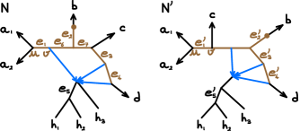
Next, we define a more stringent notion of compatibility to maintain the classification of nodes and edges as being of tree versus hybrid type, illustrated in Figs. 1 and 2.

Note that if SDAG $N^{\prime}$ is phylogenetically compatible with SDAG $N$, then $V_{T}(N)=V_{T}(N^{\prime})$ and $V_{H}(N)=V_{H}(N^{\prime})$. Note also the rooted partner of a binary network may not be binary by the typical definition for rooted networks, since the root can have degree $3$ instead of $2$.

Not all SDAGs are networks (see Fig. 1 for an example). We are interested in networks rather than general SDAGs, because a network can represent evolutionary history up to “rerooting”, as captured by its rooted partners. Fig. 1 gives an example network ($N$, top) and 2 of its 4 rooted partners (bottom).

Traditionally, phylogenetic trees and networks are connected and with a single root [30]. We consider here a broader class of graphs, allowing for multiple connected components and multiple roots per connected component. We also allow for non-simple graphs, that is, for multiple parallel edges between the same two nodes $u$ and $v$, directed and in the same direction for the graph to be acyclic. With a slight abuse of notation, we keep referring to each parallel edge as $(u,v)$. Self-loops are not allowed as they would cause the graph to be cyclic. The term “rooted partner” was introduced by Linz and Wicke [21] in the context of traditional semidirected phylogenetic networks in which the set of directed edges is precisely the set of hybrid edges, and for which a rooted partner has a single root.

We will use the following results frequently. The first one is trivial.

The next definition is motivated by the fact that phylogenies are inferred from data collected at leaves, which are known entities with labels (individuals, populations, or species), whereas non-leaf nodes are inferred and unlabeled.

Clearly, $V_{RL}(N)\subseteq V_{UL}(N)$. If $N$ is directed, then $V_{RL}(N)=V_{UL}(N)=V_{L}(N)$. As we will see later in 12, an ambiguous leaf is of degree 1 in the undirected graph obtained by undirecting all edges in $N$, hence a leaf in the traditional sense. In Fig. 2 for example, $a$ is an ambiguous leaf in $N_{1}$ but a rooted leaf in $N_{3}$.

In Section III we make no assumption regarding $V_{UL}(N)$ and $V_{RL}(N)$. But to extend $\mu$-vectors to semidirected graphs in Section IV, we will need a stable set of leaves across rooted partners. For a vector of distinct labels $\mathcal{L}$, an $\mathcal{L}$-DAG is a DAG whose leaves are bijectively labeled by $\mathcal{L}$. To extend this definition we impose $V_{UL}(N)=V_{RL}(N)$ below, but we will see (after 12) that this requirement is less stringent than it appears.

A rooted partner $G$ of an $\mathcal{L}$-network $N$ must be an $\mathcal{L}$-DAG: since $V_{RL}(N)\subseteq V_{L}(G)\subseteq V_{UL}(N)$ generally, we have that $V_{L}(G)=V_{L}(N)$ and $V_{L}(G)$ can inherit the labels in $N$.

Our main result concerns the class of tree-child graphs. If $G$ is a DAG, it is tree-child if every internal node $v$ of $G$ has at least one child that is a tree node [16]. Equivalently, $G$ is tree-child if every non-leaf node in $G$ has a tree descendant leaf [7]. We extend this notion to semidirected networks, illustrated in Fig. 2.

Since a DAG $G$ is a network with a single rooted partner, $G$ is strongly and weakly tree-child if and only if it is tree-child as a DAG. In Fig. 2, $N_{3}$ is weakly but not strongly tree-child: of its 3 rooted partners, only one is tree-child. Later in 11, we provide a characterization easy to check without enumerating rooted partners.

In a network $N$, a semidirected path from $u_{0}$ to $u_{n}$ is a sequence of nodes $u_{0}u_{1}\ldots u_{n}$, such that for $i=1,\ldots n$, either $u_{i-1}u_{i}$ or $(u_{i-1},u_{i})$ is an edge in $N$. On $V(N)$ we define $v\lesssim u$ if there is a semidirected path from $u$ to $v$, and the associated equivalence relation: $u\sim v$ if $u\lesssim v$ and $v\lesssim u$. In Fig. 2, $a\lesssim v$ in $N_{1}$ and $N_{3}$. Also $v\lesssim a$ so $a\sim v$ in $N_{1}$, but not in $N_{3}$. On equivalence classes, $\lesssim$ becomes a partial order, with which we can define the following.

The directed part of $N$ is generally not a subgraph: it may contain an edge but not one of its incident nodes. In Fig. 2, edges in the directed part $E_{DP}$ are those in black (tree edges) and blue (hybrid edges). Edges in root components $E_{R}$ are in brown. In $N_{3}$, $v$ is adjacent to the directed part, but is not in $V_{DP}(N_{3})$. $N_{2}$ has a trivial root component: $\{a\}$. The following result justifies the name given to the equivalence classes.

We now characterize undirected components as the undirected trees in the forest induced by $N$’s undirected edges.

Conceptually, a semidirected network represents uncertainty about the root(s) position. Next, we show that to resolve uncertainty, exactly 1 node from each root component must be chosen as root, and this choice can be made independently across root components. In other words, root choice functions are in one-to-one correspondence with rooted partners. As a result, all rooted partners have the same number of roots: the number of root components. In Fig. 1, $N$ has 2 root components each with 2 nodes, hence $2\times 2=4$ rooted partners.

We can define the following thanks to 7:

With as many directed edges as can be possibly implied by the directed edges in $N$, $\mathcal{C}(N)$ is the network that we are generally interested in. We define phylogenetic isomorphism between networks based on their completion.

In Fig. 2 for example, $N_{2}$ is complete, but $N_{3}$ is not. $N_{1}$ and $N_{3}$ are not phylogenetically isomorphic, because the edge incident to $a$ remains undirected in the completion $\mathcal{C}(N_{1})$. $N_{2}$ is not phylogenetically compatible with $N_{1}$ or $N_{3}$, and not phylogenetically isomorphic to either.

Using $\mathcal{C}(N)$, we can now decide if a network is weakly or strongly tree-child in a single traversal, thanks to the following.

Finally, we characterize unambiguous leaves quickly.

Formally a multiset is a tuple $(A,m)$, where $A$ is a set and $m$: $A\to\mathbb{Z}^{+}$ gives the multiplicity. We consider two multisets $(A,m_{A})$ and $(B,m_{B})$ to be the same if $m_{A}|_{A\setminus B}=0$, $m_{B}|_{B\setminus A}=0$, and $m_{A}|_{A\cap B}=m_{B}|_{A\cap B}$. To simplify notations, we use $\lbag\rbag$ to denote a multiset by enumerating each element as many times as its multiplicity. For example, $A=\lbag a,a,b\rbag$ contains $a$ with multiplicity 2 and $b$ with multiplicity 1. For brevity, we identify a multiset $(A,m)$ with the set $A$ if $m\equiv 1$, e.g. $\lbag a,b,c\rbag=\{a,b,c\}$. We adopt the standard notion of sum and difference for multisets. The symmetric difference between multisets is defined as $A\triangle B=(A-B)+(B-A)$.

In what follows, we consider a vector of distinct labels $\mathcal{L}$, whose order is arbitrary but fixed, as it will determine the order of coordinates in all $\mu$ vectors and representations. For an $\mathcal{L}$-DAG $G$ and for node $v\in V(G)$, the $\mu$-vector of $v$ is defined as the tuple $\mu(v,G)=(\mu_{1}(v),\ldots,\mu_{n}(v))$ where $n$ is the number of labels in $\mathcal{L}$ and $\mu_{i}(v)$ is the number of paths in $G$ from $v$ to the leaf with the $i^{\mathrm{th}}$ label in $\mathcal{L}$. As in [7], the partial order $\geq$ between $\mu$-vectors is the coordinatewise order. Namely, for $m=(m_{1},\ldots,m_{n})$ and $m^{\prime}=(m_{1}^{\prime},\ldots,m_{n}^{\prime})$, $m\geq m^{\prime}$ if $m_{i}\geq m_{i}^{\prime}$ for all $i=1,\ldots,n$. If $m\not\leq m^{\prime}$ and $m\not\geq m^{\prime}$ then $m$ and $m^{\prime}$ are incomparable. The node-based $\mu$-representation of $G$ from [7], denoted as $\mu_{V}(G)$, is defined as the multiset $\lbag\mu(v,G):v\in V(G)\rbag$. Algorithm 1 in [7] computes $\mu_{V}(G)$ recursively in post-order thanks to the following property, which is a slight extension of Lemma 4 in [7] allowing for parallel edges by summing over child edges instead of child nodes.

We will make frequent use of the following result, whose original proof easily extends to DAGs with parallel edges thanks to 13. It is an extension of Lemma 5 of [7] stating the assumption used in the proof by [7], which is weaker than requiring a tree-child DAG.

The rest of the section is organized as follows. In part IV-A we define the edge-based $\mu$-representation for $\mathcal{L}$-networks, with Algorithm 1 to compute it. Part IV-B presents properties of this $\mu$-representation for tree-child networks, and part IV-C describes how to reconstruct a complete tree-child $\mathcal{L}$-network from its edge-based $\mu$-representation. The networks in Fig. 3 are used as examples throughout.

References

- Allman et al. [2019] Elizabeth S. Allman, Hector Baños, and John A. Rhodes. NANUQ: a method for inferring species networks from gene trees under the coalescent model. Algorithms for Molecular Biology, 14(1), 2019. doi: 10.1186/s13015-019-0159-2.
- Ané et al. [2024] Cécile Ané, John Fogg, Elizabeth S. Allman, Hector Baños, and John A. Rhodes. Anomalous networks under the multispecies coalescent: theory and prevalence. Journal of Mathematical Biology, 88:29, 2024. doi: 10.1007/s00285-024-02050-7.
- Baños [2019] Hector Baños. Identifying species network features from gene tree quartets under the coalescent model. Bulletin of Mathematical Biology, 81(2):494–534, 2019. doi: 10.1007/s11538-018-0485-4.
- Babai [2016] László Babai. Graph isomorphism in quasipolynomial time. arXiv, 2016. doi: 10.48550/arXiv.1512.03547.
- Bai et al. [2021] Allan Bai, Péter L. Erdős, Charles Semple, and Mike Steel. Defining phylogenetic networks using ancestral profiles. Mathematical Biosciences, 332:108537, 2021. doi: 10.1016/j.mbs.2021.108537.
- Cardona et al. [2008] Gabriel Cardona, Mercè Llabrés, Francesc Rosselló, and Gabriel Valiente. A distance metric for a class of tree-sibling phylogenetic networks. Bioinformatics, 24(13):1481–1488, 2008. doi: 10.1093/bioinformatics/btn231.
- Cardona et al. [2009] Gabriel Cardona, Francesc Rosselló, and Gabriel Valiente. Comparison of tree-child phylogenetic networks. IEEE/ACM Transactions on Computational Biology and Bioinformatics, 6(4):552–569, 2009. doi: 10.1109/tcbb.2007.70270.
- Cardona et al. [2014] Gabriel Cardona, Mercè Llabrés, Francesc Rosselló, and Gabriel Valiente. The comparison of tree-sibling time consistent phylogenetic networks is graph isomorphism-complete. The Scientific World Journal, 2014:254279, 2014. doi: 10.1155/2014/254279.
- Cardona et al. [2024] Gabriel Cardona, Joan Carles Pons, Gerard Ribas, and Tomás Martínez Coronado. Comparison of orchard networks using their extended -representation. IEEE/ACM Transactions on Computational Biology and Bioinformatics, 21(3):501–507, 2024. doi: 10.1109/TCBB.2024.3361390.
- Felsenstein [2004] Joseph Felsenstein. Inferring Phylogenies. Sinauer Associates, Sunderland, Massachusetts, 2004. ISBN 0878931775. doi: 10.1086/383584.
- Gautier et al. [2022] Mathieu Gautier, Renaud Vitalis, Laurence Flori, and Arnaud Estoup. f-statistics estimation and admixture graph construction with pool-seq or allele count data using the R package poolfstat. Molecular Ecology Resources, 22(4):1394–1416, 2022. doi: 10.1111/1755-0998.13557.
- Gross et al. [2021] Elizabeth Gross, Leo van Iersel, Remie Janssen, Mark Jones, Colby Long, and Yukihiro Murakami. Distinguishing level-1 phylogenetic networks on the basis of data generated by Markov processes. Journal of Mathematical Biology, 83(3):32, 2021. doi: 10.1007/s00285-021-01653-8.
- Hickey et al. [2008] Glenn Hickey, Frank Dehne, Andrew Rau-Chaplin, and Christian Blouin. SPR distance computation for unrooted trees. Evolutionary Bioinformatics, 4:EBO.S419, 2008. doi: 10.4137/EBO.S419.
- Huber et al. [2022] Katharina T. Huber, Vincent Moulton, and Guillaume E. Scholz. Forest-based networks. Bulletin of Mathematical Biology, 84:119, 2022. doi: 10.1007/s11538-022-01081-9.
- Huber et al. [2025] Katharina T. Huber, Leo van Iersel, Vincent Moulton, and Guillaume E. Scholz. Is this network proper forest-based? Information Processing Letters, 187:106500, 2025. doi: 10.1016/j.ipl.2024.106500.
- Huson et al. [2010] Daniel H. Huson, Regula Rupp, and Celine Scornavacca. Phylogenetic Networks: Concepts, Algorithms and Applications. Cambridge University Press, Cambridge, 2010. doi: 10.1017/CBO9780511974076.
- Janssen and Murakami [2021] Remie Janssen and Yukihiro Murakami. On cherry-picking and network containment. Theoretical Computer Science, 856:121–150, 2021. doi: 10.1016/j.tcs.2020.12.031.
- Kong et al. [2022] Sungsik Kong, David L. Swofford, and Laura S. Kubatko. Inference of phylogenetic networks from sequence data using composite likelihood. bioRxiv, 2022. doi: 10.1101/2022.11.14.516468.
- Kuhn [1955] Harold W. Kuhn. The hungarian method for the assignment problem. Naval Research Logistics Quarterly, 2(1-2):83–97, 1955. doi: 10.1002/nav.3800020109.
- Kuhner and Felsenstein [1994] M K Kuhner and J Felsenstein. A simulation comparison of phylogeny algorithms under equal and unequal evolutionary rates. Molecular Biology and Evolution, 11(3):459–468, 1994. doi: 10.1093/oxfordjournals.molbev.a040126.
- Linz and Wicke [2023] Simone Linz and Kristina Wicke. Exploring spaces of semi-directed level-1 networks. Journal of Mathematical Biology, 87(70), 2023. doi: 10.1007/s00285-023-02004-5.
- Lutteropp et al. [2022] Sarah Lutteropp, Celine Scornavacca, Alexey M Kozlov, Benoit Morel, and Alexandros Stamatakis. NetRAX: accurate and fast maximum likelihood phylogenetic network inference. Bioinformatics, 38(15):3725–3733, 2022. doi: 10.1093/bioinformatics/btac396.
- Maier et al. [2023] Robert Maier, Pavel Flegontov, Olga Flegontova, Ulaş Işıldak, Piya Changmai, and David Reich. On the limits of fitting complex models of population history to f-statistics. eLife, 12:e85492, 2023. doi: 10.7554/eLife.85492.
- Martin et al. [2023] Samuel Martin, Vincent Moulton, and Richard M. Leggett. Algebraic invariants for inferring 4-leaf semi-directed phylogenetic networks. bioRxiv, 2023. doi: 10.1101/2023.09.11.557152.
- Neureiter et al. [2022] Nico Neureiter, Peter Ranacher, Nour Efrat-Kowalsky, Gereon A. Kaiping, Robert Weibel, Paul Widmer, and Remco R. Bouckaert. Detecting contact in language trees: a Bayesian phylogenetic model with horizontal transfer. Humanities and Social Sciences Communications, 9(1):205, 2022. doi: 10.1057/s41599-022-01211-7.
- Robinson and Foulds [1979] D. F. Robinson and L. R. Foulds. Comparison of weighted labelled trees. In A. F. Horadam and W. D. Wallis, editors, Combinatorial Mathematics VI, pages 119–126, Berlin, Heidelberg, 1979. Springer Berlin Heidelberg. ISBN 978-3-540-34857-3.
- Robinson and Foulds [1981] D.F. Robinson and L.R. Foulds. Comparison of phylogenetic trees. Mathematical Biosciences, 53(1):131–147, 1981. doi: doi.org/10.1016/0025-5564(81)90043-2.
- Solís-Lemus and Ané [2016] Claudia Solís-Lemus and Cécile Ané. Inferring phylogenetic networks with maximum pseudolikelihood under incomplete lineage sorting. PLOS Genetics, 12(3):e1005896, 2016. doi: 10.1371/journal.pgen.1005896.
- Soraggi and Wiuf [2019] Samuele Soraggi and Carsten Wiuf. General theory for stochastic admixture graphs and f-statistics. Theoretical Population Biology, 125:56–66, 2019. doi: 10.1016/j.tpb.2018.12.002.
- Steel [2016] Mike Steel. Phylogeny: Discrete and Random Processes in Evolution. Society for Industrial and Applied Mathematics, Philadelphia, PA, 2016. doi: 10.1137/1.9781611974485.
- Vachaspati and Warnow [2017] Pranjal Vachaspati and Tandy Warnow. Fastrfs: fast and accurate Robinson-Foulds supertrees using constrained exact optimization. Bioinformatics, 33(5):631–639, 2017. doi: 10.1093/bioinformatics/btw600.
- van Iersel et al. [2022] Leo van Iersel, Remie Janssen, Mark Jones, and Yukihiro Murakami. Orchard networks are trees with additional horizontal arcs. Bulletin of Mathematical Biology, 84:76, 2022. doi: 10.1007/s11538-022-01037-z.
- Xu and Ané [2023] Jingcheng Xu and Cécile Ané. Identifiability of local and global features of phylogenetic networks from average distances. Journal of Mathematical Biology, 86(1):12, 2023. doi: 10.1007/s00285-022-01847-8.
- Zhang et al. [2018] Chao Zhang, Maryam Rabiee, Erfan Sayyari, and Siavash Mirarab. ASTRAL-III: polynomial time species tree reconstruction from partially resolved gene trees. BMC Bioinformatics, 19(Suppl 6):153, 2018. doi: 10.1186/s12859-018-2129-y.
[Example edge-based -representation]
Let . In Fig. 3 left, is an -network. In -vectors, leaves are ordered as in . Following notations in Algorithm 1, where the multisets () partition the -vector sets based on their type (uni/bidirectional) and tags (, or ).
contains the -vector sets of tree edges in the directed part (in black in Fig. 3), which are here the pendent edges (incident to leaves) and :