A direct importance sampling-based framework for rare event uncertainty quantification in non-Gaussian spaces
Abstract
This work introduces a novel framework for precisely and efficiently estimating rare event probabilities in complex, high-dimensional non-Gaussian spaces, building on our foundational Approximate Sampling Target with Post-processing Adjustment (ASTPA) approach. An unnormalized sampling target is first constructed and sampled, relaxing the optimal importance sampling distribution and appropriately designed for non-Gaussian spaces. Post-sampling, its normalizing constant is estimated using a stable inverse importance sampling procedure, employing an importance sampling density based on the already available samples. The sought probability is then computed based on the estimates evaluated in these two stages. The proposed estimator is theoretically analyzed, proving its unbiasedness and deriving its analytical coefficient of variation. To sample the constructed target, we resort to our developed Quasi-Newton mass preconditioned Hamiltonian MCMC (QNp-HMCMC) and we prove that it converges to the correct stationary target distribution. To avoid the challenging task of tuning the trajectory length in complex spaces, QNp-HMCMC is effectively utilized in this work with a single-step integration. We thus show the equivalence of QNp-HMCMC with single-step implementation to a unique and efficient preconditioned Metropolis-adjusted Langevin algorithm (MALA). An optimization approach is also leveraged to initiate QNp-HMCMC effectively, and the implementation of the developed framework in bounded spaces is eventually discussed. A series of diverse problems involving high dimensionality (several hundred inputs), strong nonlinearity, and non-Gaussianity is presented, showcasing the capabilities and efficiency of the suggested framework and demonstrating its advantages compared to relevant state-of-the-art sampling methods.
Keywords Rare Event Non-Gaussian Inverse Importance Sampling Reliability Estimation Hamiltonian MCMC Quasi-Newton Preconditioned MALA High dimensions.
1 Introduction
This work introduces a new framework for directly estimating rare event probabilities in complex, high-dimensional non-Gaussian spaces. Rare event uncertainty quantification is a pivotal component in contemporary decision-making across diverse domains. It is particularly crucial for assessing and mitigating risks tied to infrequent yet highly impactful rare event occurrences, such as structural failures induced by extreme loads like earthquakes and hurricanes. This field, commonly referred to as reliability estimation in engineering, has a long history, and comprehensive insights into its complexities can be read in [1, 2, 3, 4, 5, 6]. In many practical applications, rare event probabilities are fortunately exceptionally low, often within the range of to even and lower, posing significant numerical and mathematical challenges. Further complicating these challenges is the reliance on computationally expensive models of the involved systems with high-dimensional random variable spaces. Achieving accurate estimates while minimizing model evaluations is thus a critical parameter.
Numerous existing solution techniques are specifically designed for Gaussian spaces and typically seek to transform non-Gaussian random variables to Gaussian ones. However, when such Gaussian transformations are not possible, these techniques often encounter challenges in non-Gaussian spaces due to potential asymmetries, complex dependencies, intricate geometries, and constrained spaces. Approximation methods, such as First Order Reliability Method (FORM) [7, 8], Second Order Reliability Method (SORM) [9], and Large deviation theory (LDT) [10, 11, 12], provide asymptotic expressions for estimating rare event probabilities [13]. In general, these methods lose accuracy and/or practicality for arbitrary non-Gaussian distributions, and may also exhibit considerable errors in problems with moderately to highly nonlinear performance functions [7, 14]. Sampling methods can tackle the problem in its utmost generality, however, with a higher computational cost. In addressing the known limitations of the crude Monte Carlo approach [15], numerous sophisticated sampling methods have been proposed. Among others, the Subset Simulation (SuS) approach, originally presented in [16], has been widely used and continuously enhanced for Gaussian spaces [17, 18, 19, 20], given its potential to handle high-dimensional problems, despite some limitations [21]. Several more recent works have also shown enhanced performance in non-Gaussian spaces by mainly employing advanced samplers within SuS, such as Hamiltonian MCMC [22, 23], Riemannian Manifold Hamiltonian Monte Carlo (RMHMC) [24, 25], Hamiltonian Neural Networks (HNN) [26], and affine invariant ensemble MCMC sampler [27, 28]. It should be noted that Subset Simulation also has similarities with multilevel splitting methods [29, 30, 31]. Another sampling method capable of efficiently estimating rare event probabilities is importance sampling (IS), a well-known variance-reduction approach. Since this work builds upon the theoretically rigorous foundations of importance sampling, we provide a comprehensive review and discussion of IS techniques for rare event estimation in Section 2. Combining surrogate models, that approximate computationally expensive original models, with sampling-based approaches has also demonstrated significant savings in computational cost across various applications [32, 33, 34]; however, their applicability to high-dimensional, complex problems still faces practical challenges.
In this paper, we introduce a novel framework for efficiently and precisely estimating rare event probabilities, directly in non-Gaussian spaces, building on our foundational Approximate Sampling Target with Post-processing Adjustment (ASTPA) approach, recently developed for Gaussian spaces in [35]. As shown in this work, the developed framework demonstrates excellent performance in challenging high-dimensional non-Gaussian scenarios, thereby overcoming a significant limitation of numerous existing methods. In essence, rare event probability estimation is a normalizing constant estimation problem for the joint distribution of the involved random variables truncated over the rare event domain, also known as the optimal sampling target; a demanding problem traditionally approached through sequential techniques. Conversely, the ASTPA approach directly and innovatively addresses this challenge by decomposing the problem into two less demanding estimation problems. Hence, the proposed methodology first constructs an unnormalized sampling target, appropriately designed for non-Gaussian spaces, relaxing the optimal importance sampling distribution. To sample this constructed target adequately, our Quasi-Newton mass preconditioned Hamiltonian MCMC (QNp-HMCMC) algorithm is employed, particularly suitable for complex spaces, as discussed later. The obtained samples are subsequently utilized not only to compute a shifted estimate of the sought probability but also to guide the second ASTPA stage. Post-sampling, the normalizing constant of the approximate sampling target is computed through the inverse importance sampling (IIS) technique [35], which utilizes an importance sampling density (ISD) fitted based on the samples drawn in the first stage. A practical approach augmenting the IIS stability in challenging non-Gaussian settings, by avoiding anomalous samples, is also devised in this work. The rare event probability is eventually computed by utilizing this computed normalizing constant to correct the shifted estimate of the first stage. The statistical properties of the proposed estimator are thoroughly derived, including its proven unbiasedness and analytical coefficient of variation (C.o.V). Notably, the derived analytical C.o.V expression, accompanied by an applied implementation technique based on the effective sample size, has demonstrated accurate agreement with numerical results.
Hamiltonian Markov Chain Monte Carlo (HMCMC) is one of the most successful and powerful MCMC algorithms [22, 36], based, as the name suggests, on Hamiltonian dynamics [37]. Its performance largely depends on tuning three parameters: the mass matrix, the simulation step size, and the length of the simulated trajectories. Its efficiency in high-dimensional complex spaces can be significantly improved by selecting an appropriate mass matrix [24, 38, 39]. Therefore, in this work, we rigorously analyze a Quasi-Newton mass preconditioned HMCMC (QNp-HMCMC) sampling algorithm, an approach we initially conceptualized in our earlier work [35]. QNp-HMCMC effectively and uniquely leverages the geometric information of the target distribution. During the burn-in stage, a skew-symmetric preconditioning scheme for the Hamiltonian dynamics is adopted [40], incorporating Hessian information merely approximated based on the already available gradients. The estimated Hessian is subsequently utilized to provide an informed, preconditioned mass matrix, better describing the scale and correlation of the involved random variables. To reinforce its theoretical basis, we prove here that simulating the skew-symmetric preconditioned dynamics in QNp-HMCMC leads to the correct stationary target distribution. To effectively implement QNp-HMCMC, we provide detailed recommendations for approximating the Hessian information in complex non-Gaussian spaces. The simulation step size in QNp-HMCMC is automatically tuned using the dual averaging algorithm [41, 42]. Equipped with the preconditioned dynamics and mass matrix, QNp-HMCMC is characterized by large informed sampling steps, enabling it to work efficiently even with single-step simulated Hamiltonian dynamics, avoiding the challenging task of tuning its trajectory length in general, intricate domains, and enabling increased computational efficiency by minimizing the number of model calls (gradient evaluations). As proven in this work, this QNp-HMCMC version with a single-step implementation is equivalent to an original preconditioned Metropolis-adjusted Langevin algorithm (MALA). Finally, an optimization approach is also devised in this paper to initiate the QNp-HMCMC sampling effectively.
This paper is structured as follows. Section 2 offers a comprehensive discussion on existing importance sampling-based methods for rare event probability estimation, highlighting their common characteristics and, notably, their connections and differences with our ASTPA approach. The developed framework is subsequently presented in Section 3, and Section 4 discusses in detail the single-step QNp-HMCMC algorithm. Section 5 introduces an effective optimization approach for rare event domain discovery, specifically using the Adam optimizer [43], aiming to provide good initial states for the MCMC sampler. Given that it is more practical for MCMC and HMCMC algorithms to operate in unconstrained spaces, Section 6 discusses transforming bounded random variables to unconstrained ones. A summary of the QNp-HMCMC-based ASTPA framework for non-Gaussian domains is then presented in Section 7. To fully examine the capabilities of the proposed methodology, in Section 8 its performance is demonstrated and successfully compared against the state-of-the-art Subset Simulation, and related variants, in a series of challenging low- and high-dimensional non-Gaussian problems. The paper then concludes in Section 9.
2 Rare Event Probability Estimation
Let be a continuous random vector taking values in and having a joint probability density function (PDF) . We are interested in rare events , where is a performance function, also known as the limit-state function, defining the occurrence of a rare event. In the context of reliability estimation, which considers failures as rare events, the limit state function, for example, can be formulated as , where denotes a model output (a quantity of interest). Here, the predefined threshold determines the rarity of the failure event by controlling when starts to take non-positive values, i.e., rare event occurrence. In this work, we aim to estimate the rare event probability :
| (1) |
where is the indicator function, i.e., if , and otherwise, and is the expectation operator.
Our objective in this work is to estimate the described integration in Eq. 1 under these challenging yet realistic settings: (i) the analytical calculation of Eq. 1 is generally intractable, as the limit-state function can be complicated, e.g., involve the solution of a differential equation; (ii) the computational effort for evaluating for each realization is assumed to be quite significant, often relying on computationally intensive models, necessitating the minimization of such function evaluations (model calls); (iii) the rare event probability is extremely low, e.g., in order of ; (iv) the random variable space, , is assumed to be high-dimensional, e.g., and more; (v) the joint probability density, , is non-Gaussian, with transformations to the Gaussian domain assumed inapplicable, necessitating Eq. 1 evaluation directly in non-Gaussian spaces.
Under these settings, several sampling methods become highly inefficient and fail to address the problem effectively. For instance, the standard Monte Carlo estimator of Eq. 1 using draws from , , has a coefficient of variation , rendering this estimate inefficient by requiring a prohibitively large number of samples to accurately quantify small probabilities; see setting (iii) above. Importance sampling (IS), as a variance-reduction method, can efficiently compute the integral in Eq. 1, through sampling from an appropriate importance sampling density (ISD), . The ISD places greater importance on rare event domains in the random variable space compared to , satisfying the sufficient condition , with denoting the support of the function. This results in an increased number of rare event samples, thereby reducing the number of required model calls. Eq. (1) can then be written as:
| (2) |
leading to the unbiased IS estimator:
| (3) |
The efficiency of IS relies heavily on the careful selection of both the ISD and the sampling algorithm. A theoretically optimal ISD , providing zero-variance IS estimator, can be given as [44]:
| (4) |
Yet, it is evident that this ISD cannot be utilized due to the fact that the normalizing constant in Eq. (4) is the sought target probability . Notably, finding a near-optimal ISD, approximating , is an ongoing research pursuit. The existing approaches can be largely classified into two categories. The first directly follows the IS estimator in Eq. 3 and seeks to approximate by a parametric or non-parametric probability density function (PDF), . An early approach in this category utilizes densities centered around one or more design points [45], provided by an initial FORM analysis, which has later been deemed ineffective for high-dimensional, complex spaces [16]. A more recent popular approach is the cross entropy-based importance sampling (CE-IS). It alternatively constructs a parametric ISD by minimizing the Kullback-Leibler (KL) divergence between and a chosen parametric family of probability distributions [46, 47, 48, 49, 50]. Recent CE-IS variants incorporate information from influential rare event points, e.g., design points, to effectively initialize the cross entropy process [51, 52]. Within this first category of methods, several different noteworthy approaches have also been proposed to approximate , e.g., [53, 54, 55, 56, 57].
Before delving into the second category of methods, we define ISD , where is an unnormalized importance distribution, and is its normalizing constant. Following this definition, denotes an unnormalized optimal importance sampling distribution, and is its normalizing constant. Thus, in the second category of methods, sequential variants of importance sampling are employed, mainly utilizing a number of intermediate unnormalized distributions. These unnormalized distributions are generally more flexible than the PDFs usually utilized within the first category, as discussed above, thus being capable of providing a better approximation of . Employing an unnormalized importance sampling distribution , Eq. 2 can be written as:
| (5) |
Existing methods currently compute the normalizing constant, , using consecutive intermediate unnormalized distributions ’s, , following Eq. 6. These distributions should be designed to link between and , with and being the closest to and , respectively.
| (6) |
where is the normalizing constant of , and , typically, is the normalizing constant of the original distribution . is left in Eq. 6 for generality purposes, particularly to cover scenarios when an unnormalized original distribution is instead provided (substitute in Eq. 5 to verify that). Eq. 6 can be computed using the sequential importance sampling (SIS) approach as [58, 59]:
| (7) |
Alternatively, bridge sampling can evaluate Eq. 6 as [60, 61, 62]:
| (8) |
where is a bridge distribution [61] between and , and is its associated normalizing constant. This latter technique aims to provide a more accurate estimate even if the two consecutive distributions, and , are not close enough. Eq. 6 can also be computed using path sampling [63, 64]. A key to the success of these sequential methods is to design nearby intermediate distributions and to sufficiently sample them to accurately compute Eq. 6, a non-trivial and computationally demanding task. A discussion on methods within this second category can be found in [65]. Interestingly, the subset simulation method [16] can also be seen as a special case of this second category, wherein the ratio is the conditional probability between every two consecutive intermediate events, and .
In this work, we are originally estimating Eq. 5 in a non-sequential manner, using a single unnormalized distribution , approximating , i.e., . Therefore, the proposed approach significantly reduces the computational cost associated with employing multiple intermediate distributions. The discovery of the rare event domain is alternatively achieved through the utilization of advanced samplers and optimization techniques, as detailed in Section 5. It should also be noted that the discussed importance sampling-based methods in the current literature are mostly tailored for Gaussian spaces. Consequently, the ability of our proposed framework to operate directly in non-Gaussian spaces is an additional substantial benefit.
3 Approximate Sampling Target with Post-processing Adjustment (ASTPA) in Non-Gaussian Spaces
ASTPA estimates the rare event probability in Eq. 1 through an innovative non-sequential importance sampling variant evaluating Eq. 5. To this end, ASTPA constructs a single unnormalized approximate sampling target , relaxing the optimal ISD in Eq. 4. Post-sampling, its normalizing constant is computed utilizing our devised inverse importance sampling. For clarity, we rewrite Eq. 5 as:
| (9) |
Computing is thus decomposed into two (hopefully simpler) problems. The first involves constructing and sampling , to compute the unbiased expectation of the weighted indicator function (shifted probability estimate) as:
| (10) |
An empirical estimation for the normalizing constant, , is then computed using the inverse importance sampling, as discussed in Section 3.2. The ASTPA estimator for the sought rare event probability can then be computed as:
| (11) |
Fig. 1 concisely portrays the proposed framework using a correlated Gumbel distribution and a quadratic limit state function, as detailed in Section 8.1, with . The construction of the approximate sampling target in ASTPA is discussed in Section 3.1, including its recommended parameters for problems described in non-Gaussian spaces. Then, we present the inverse importance sampling approach in Section 3.2. Subsequently, Section 3.3 discusses thoroughly the statistical properties of the proposed estimator presented in Eq. 11.
 |

|
|||
| (a) | (b) | |||

|

|

|
|
|
| (c) | (d) Samples | (e) | (f) Samples |
3.1 Target distribution formulation
As discussed earlier, the basic idea is to construct a near-optimal sampling target distribution , placing higher importance on the rare event domain . Similar to methods utilizing sequential variants of IS (see Section 2 for details), the approximate sampling target in ASTPA is constructed by approximating the indicator function with a smooth function, namely a likelihood function . This likelihood function is chosen as a logistic cumulative distribution function (CDF) of the negative of a scaled limit state function, , with being a scaling constant:
| (12) |
where and are the mean and dispersion factor of the logistic CDF, respectively; their recommended values are subsequently discussed. Our numerical experiments in this work and [35] have underscored the effectiveness of this chosen approximation of . It should also be noted, however, that there exist numerous choices for approximating in the literature, e.g., standard normal CDF [59, 48], and exponential tilting barrier [62]. The approximate sampling target is ASTPA is then expressed as:
| (13) |
The scaling is suggested to handle the varying magnitudes that different limit-state functions can exhibit. It is implemented in a way ensuring that the input to the logistic CDF at an influential point with respect to the original distribution consistently falls within a predefined range, regardless the magnitude of . In this work, we use the mean value of the original distribution, , to represent this influential point, albeit other points could also serve this purpose. To make the input to the logistic CDF, when evaluated at , lies in a desired range of , we define as:
| (14) |
For example, if , this scaling ensures that the input at equals , i.e., . Fine-tuning values of the scaling constant, , within the recommended range is not usually necessary. Our empirical investigation has confirmed the effectiveness of this proposed scaling technique and demonstrated that the recommended range for is practical for the studied non-Gaussian problems.
The dispersion factor of the logistic CDF, , determines the widespread of the likelihood function, thus controlling the shape of the constructed target . For non-Gaussian spaces, values are recommended in the range . Fine-tuning higher decimal values of in that range is not usually necessary. Lower values, , usually work efficiently, whereas a higher value within the recommended range may be needed for cases involving a large number of (strongly) nonlinear random variables.
For the mean parameter, , of the logistic CDF, , we are interested in generally locating it inside the rare event domain, , to enhance the sampling efficiency. As such, we are describing through a percentile, , of the logistic CDF and its quantile function, :
| (15) |
By placing a chosen percentile of the logistic CDF on the limit-state surface at , the mean parameter can be computed as:
| (16) |
Based on our empirical investigation, we found that using the percentile () yields good efficiency. Therefore, it is used in all our experiments in this work. Substituting in Eq. 16, the mean parameter is then defined as a function of the dispersion factor as .

|

|

|
|

|

|

|
In Fig. 2, we illustrate how the likelihood dispersion factor, , and the scaling constant, , influence the shape of the target distribution, based on a correlated Gumbel distribution, as detailed in Section 8.1. As can be seen, decreasing and/or increasing results in a more concentrated target distribution inside the rare event domain. Although an increasing number of rare event samples can be obtained by pushing the target further inside the rare event domain, i.e., being very close to the optimal one , that may also complicate the sampling process and the computation of the normalizing constant , as discussed in Section 3.4.
3.2 Inverse Importance Sampling
Inverse importance sampling (IIS) is a general technique to compute normalizing constants, demonstrating exceptional performance in the context of rare event probability estimation. Given an unnormalized distribution , and samples , inverse importance sampling first fit an ISD based the samples ; details of is discussed below. IIS then estimates the normalizing constant as:
| (17) |
By drawing i.i.d. samples from , the unbiased normalizing constant estimator can be computed as:
| (18) |
In this work, the ISD is a computed Gaussian Mixture Model (GMM), based again on the already available samples, , and the generic Expectation-Maximization (EM) algorithm [66]. A typical GMM expression can be then given by:
| (19) |
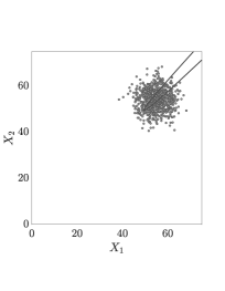
where is the PDF, is the weight, is the mean vector and is the covariance matrix of the Gaussian component, that can all be estimated, for all components, by the EM algorithm. In low-dimensional spaces, where , we employ a GMM with a large number of Gaussian components that have full covariance matrices. This approach aims to accurately approximate the target distribution with an ISD , thus improving the IIS estimator in Eq. 18. In contrast, for higher dimensions, we fit Gaussian Mixture Models (GMMs) with diagonal covariance matrices. That is to reduce the number of GMM parameters to be estimated, thereby mitigating the scalability issues commonly associated with GMMs. Specifically, for high-dimensional examples discussed in this paper, we utilize a GMM fitted with a single component and a diagonal covariance matrix, i.e., a multivariate independent Gaussian density. This method has demonstrated exceptional efficacy in calculating the normalizing constant for challenging examples, even in spaces with dimensions as high as 500. Notably, this IIS technique can generally still work effectively even using a crudely fitted . We demonstrate this feature by employing two different choices for the ISD, , to quantify the target probability in the illustrative example depicted in Fig. 1, with . The first is an accurate GMM with ten Gaussian components having full covariance matrices, as depicted in Fig. 3 , which yields of and a coefficient of variation (C.o.V) of . On the other hand, using the same number of total model calls (), the crudely fitted GMM in Fig. 1(e) still provides very good performance with an estimated probability of and a C.o.V of . The ASTPA estimator of the rare event probability can finally be computed as:
| (20) |
where and are samples from and , respectively.
 |
 |
| (a) | (b) Samples |
Remark 1.
We introduce an effective approach to enhance the robustness of the IIS estimator against the impact of rarely observed outlier or anomalous samples. Initially, the sample set is split into two subsets of equal size: and , given that is an even number. Subsequently, Eq. 18 is computed separately for each subset, yielding two estimates, and . If these two estimates fall within a reasonable range of each other, specifically if , we then compute the final IIS estimate as their average, . This is equivalent to compute Eq. 18 using the entire set . However, in rare cases, the estimates diverge beyond this threshold, indicating potential instability, and a conservative approach is thus adopted. In these instances, the final estimator is determined as the minimum of the two estimates, . This method has been successfully applied in all examples presented in this work.
3.3 Statistical properties of the ASTPA estimator ()
In this section, we show unbiasedness and the analytical Coefficient of Variation (C.o.V) of the ASTPA estimator, , in Eq. 20. Assuming and are independent, the expected value of their product can be expressed as:
| (21) |
Considering their formulation in Eqs. 10 and 18, and are unbiased estimators of and , respectively, i.e., and . The ASTPA estimator is thus unbiased:
| (22) |
The variance () of the ASTPA estimator can then be computed as:
| (23) |
where and can be computed according to Eqs. 10 and 18, respectively. and can thus be estimated as follows:
| (24) |
| (25) |
where and are samples from and , respectively. denotes the number of used Markov chain samples, taking into account the fact that the samples are not independent and identically distributed (i.i.d) in this case. The analytical Coefficient of Variation (C.o.V) can then be provided as:
| (26) |
In this work, the thinning process reduces the sample size from to based on the effective sample size (ESS) of the sample set . We select every sample for thinning, where , an integer, is determined by:
| (27) |
where represents the minimum effective sample size across all dimensions and is computed using TensorFlow Probability software [67]. To ensure remains within practical bounds for the thinning process, it is constrained to the set , with any calculated value of outside this range being adjusted to the nearest bound within it. The analytical C.o.V computed according to this approach showed good agreement with the sample C.o.V in all our numerical examples.
Remark 2.
The unbiasedness of the ASTPA estimator is based on assuming independence between and . If dependence exists, the expected value of their product becomes:
| (28) |
where is the covariance between and . This dependence could arise from using the sample set to fit the ISD , leading to a potential bias in the estimator. Despite this potential for bias, our empirical investigations using a finite sample size reveal that the bias of the ASTPA estimator is minimal. One approach to ensure independence, if wanted, is to fit the ISD on an additional sample set , separate from the one used to estimate . Our empirical findings, however, suggest that such steps are generally unnecessary.
3.4 Impact of the constructed sampling target on the estimated probability
In this section, we illustrate how constructing the sampling target, , influences the estimated probability . To this end, we consider three cases: (a) a highly relaxed target using and values outside the recommended ranges, (b) a target constructed with and values within the recommended ranges, and (c) a target highly concentrated inside the rare event domain, i.e., very close to the theoretically optimal ISD in Eq. 4. We again consider the correlated Gumbel distribution example, as detailed in Section 8.1, with . Fig. 4 depictes these three constructed targets, accompanied by the corresponding and values. The impact on the estimator accuracy is judged using the sampling coefficients of variation (C.o.V) of the normalizing constant (Eq. 18), the shifted probability estimate (Eq. 10), and the sought probability (Eq. 20), as well as the expected values of . Fig. 4 shows the results obtained using a total number of model calls in all cases and based on 100 independent simulations.
In Fig. 4(a), the highly relaxed target is mainly located outside the rare event domain, thus resulting in a low number of rare event samples. Therefore, the C.o.V of becomes high since only a few samples with appear in Eq. 10. Conversely, the case shown in Fig. 4(b) demonstrates excellent performance with low coefficients of variation and very close to the reference value. On the other hand, the highly concentrated target in Fig. 4(c), constructed using and values outside the recommended range, presents interesting results with an approximately zero C.o.V for , and a comparatively higher C.o.V of . The reason for the former is that almost all the samples yield , therefore regardless of the number of samples. However, this concentrated sampling target may not often be sampled adequately using an affordable number of model calls compared to an appropriately relaxed target. Consequently, the fitted GMM within the inverse importance sampling procedure may not accurately represent the target . The accuracy of the estimated normalizing constant then slightly deteriorates in this 2-dimensional example. This decrease in accuracy becomes significantly more pronounced if the scenario in Fig. 4(c) is followed in high-dimensional problems, e.g., the high-dimensional examples discussed in Section 8.
The deteriorated performance observed sometimes in certain importance sampling-based methods, particularly for high-dimensional and significantly nonlinear performance functions, can be attributed to the scenario outlined in Fig. 4(c). Specifically, some methods, see [53, 55] for example, aim to sample the unnormalized optimal distribution , and then fit a normalized PDF based on these samples. Another sample set from the fitted PDF is then employed to compute the normalizing constant of , which is the sought probability . This investigation here, therefore, underscores the sampling benefits of appropriately relaxing (smoothing) the indicator function, often leading to enhanced performance.

|

|

|
|
|---|---|---|---|
| (a) | (b) | (c) | |
| C.o.V | 0.40 | 0.03 | 0.00 |
| C.o.V | 0.13 | 0.02 | 0.13 |
| C.o.V | 0.40 | 0.03 | 0.13 |
| 2.38E-7 | 2.52E-7 | 2.33E-7 |
4 Sampling the Approximate Target () in ASTPA
In this section, we discuss sampling the approximate target in ASTPA using gradient-based Markov Chain Monte Carlo (MCMC) methods. Specifically, we focus on the state-of-the-art Hamiltonian MCMC (HMCMC) methods, including our developed Quasi-Newton mass preconditioned HMCMC (QNp-HMCMC), aimed at improving sampling efficiency for intricate probability distributions. We first present the standard HMCMC algorithm, followed by our developed QNp-HMCMC, emphasizing its theoretical foundations and practical implementation techniques for complex non-Gaussian spaces. Connections with the preconditioned Metropolis-adjusted Langevin algorithm (MALA) are illustrated, highlighting the uniqueness of QNp-HMCMC, even with a single-step integration.
4.1 Hamiltonian Markov Chain Monte Carlo (HMCMC)
HMCMC leverages Hamiltonian dynamics to generate distant Markov chain samples, thereby avoiding the slow exploration of high-dimensional random variable spaces encountered in random-walk samplers. This Hamiltonian approach was first introduced to molecular simulations by Alder and Wainwright in [68], in which the motion of the molecules was deterministic. Subsequently, Duane et al. [37] integrated MCMC methods with molecular dynamics approaches. The enhanced sampling efficiency of HMCMC is mainly attributed to the augmentation of the space with momentum variables and the utilization of the target distribution’s gradient, facilitating informed sampling steps.
Given -dimensional variables of interest with unnormalized density (.), HMCMC introduces -dimensional auxiliary momentum variables and then samples from the joint distribution characterized by:
| (29) |
where is termed the Hamiltonian function . The functions and are introduced as the potential energy and kinetic energy, owing to the concept of the canonical distribution [22] and the physical laws which motivate the Hamiltonian Markov Chain Monte Carlo algorithm. The kinetic energy function is unconstrained and can be formed in various ways according to the implementation. In most typical cases, the momentum is sampled by a zero-mean normal distribution [22, 69], and accordingly, the kinetic energy can be written as , where is a symmetric, positive-definite matrix, termed mass matrix. The joint distribution can then be written as:
| (30) |
where denotes a Gaussian distribution. HMCMC generates a Metropolis proposal on the joint state-space by sampling the momentum and simulating trajectories of Hamiltonian dynamics in which the time evolution of the state is governed by Hamilton’s equations, expressed typically by:
| (31) |
where denotes here the log-density of the target distribution. Hamiltonian dynamics prove to be an effective proposal generation mechanism because the distribution is invariant under the dynamics of Eq. 31. These dynamics enable a proposal, triggered by an approximate solution of Eq. 31, to be distant from the current state, yet with high probability acceptance. The solution to Eq. 31 is analytically intractable in general and thus the Hamiltonian equations need to be numerically solved by discretizing time using some small step size, . A symplectic integrator that can be used for the numerical solution is the leapfrog one and works as follows:
| (32) |
where and . The main advantage of using the leapfrog integrator is its simplicity, that is volume-preserving, and that it is reversible, due to its symmetry, by simply negating , in order to generate a valid Metropolis proposal. See Neal [22] and Betancourt [69] for more details on energy-conservation, reversibility and volume-preserving integrators and their connections to HMCMC. It is noted that in the above leapfrog integration algorithm, the computationally expensive part is the one model call per step to acquire the term. With the trajectory or else path length, taking leapfrog steps approximates the evolution , providing the exact solution in the limit . Section 4.3 discusses techniques for tuning these parameters.
A generic procedure for drawing samples via HMCMC is described in Algorithm 1, where again is the log-density of the target distribution of interest, are initial values, and L is the number of leapfrog steps, as explained before. For each HMCMC step, the momentum is first resampled, and then the L leapfrog updates are performed, as seen in Eq. 32, before a typical accept/reject Metropolis step takes place. In Algorithm 1, the mass matrix M is set to the identity matrix, I, as often followed in the standard implementation of HMCMC. However, the efficiency of the HMCMC can be significantly enhanced by appropriately selecting the mass matrix, particularly when dealing with complex, high-dimensional distributions. In the subsequent section, we introduce our developed technique for adapting the mass matrix, which has shown substantial improvement in the sampling efficiency.
4.2 Quasi-Newton mass preconditioned HMCMC (QNp-HMCMC)
In complex, high-dimensional problems, the performance of the standard HMCMC sampler, presented as Algorithm 1, may deteriorate, necessitating a prohibitive number of model calls. Various strategies have been proposed to overcome this limitation, including the adaptation of the mass matrix , as highlighted in [24, 38, 39, 70]. We have uniquely employed this technique in our Quasi-Newton mass preconditioned HMCMC (QNp-HMCMC), as presented in Algorithm 2 and discussed in this section. The role of the mass matrix in HMCMC is analogous to performing a linear transformation for the involved random variables , potentially simplifying the geometric complexity of the underlying sampling distribution. Such a transformation may thus make the transformed variables less correlated and have a similar scale, facilitating a more efficient sampling process. Specifically, operating HMCMC in a transformed space , where is a non-singular matrix, and using a standard mass matrix is equivalent to using a transformed mass matrix in the original space [22, 38].
The mass matrix is commonly adapted to better describe the local geometry of the target distribution, enabling more efficient exploration of the space of random variables. For instance, the Riemannian Manifold Hamiltonian Monte Carlo (RMHMC) approach, suggested in [24], leverages the manifold structure of the variable space through a position-specific Riemannian metric tensor. This tensor functions as a position-dependent mass matrix, leading to a non-separable Hamiltonian. Therefore, solving the Hamiltonian equations within RMHMC requires a generalized leapfrog scheme, demanding higher-order derivatives of distributions and additional model calls per leapfrog step. Conversely, within the scope of our research, a more computationally feasible approach is to introduce a position-independent mass matrix , as in algorithm 1, describing the local structure of the target distribution. Such description can be generally obtained in a Newton-type context utilizing the Hessian information of the target distribution, as demonstrated in various MCMC methods [71, 72, 73, 74]. In the context of HMCMC, Zhang and Sutton [38] employed a quasi-Newton-type approach to provide a position-independent, yet continuously adapted, mass matrix using a variant of the BFGS formula [75] to approximate the Hessian matrix. They maintained position independence by adopting the ensemble chain adaption (ECA) approach [76], updating the mass matrix for each chain based on the states of others. In QNp-HMCMC, we utilize an alternative approach to ensure position independence by approximating the Hessian matrix during a burn-in phase and subsequently utilizing it as a constant mass matrix. Importantly, we enhance the burn-in stage’s efficiency through a skew-symmetric preconditioning approach while setting the mass matrix to identity.
In this work, we approximate the Hessian information of the potential energy function, , using the well-known BFGS approximation [77], solely based on the gradient information. Let , consistent with the previous sections. Given the - estimate , where is an approximation to the inverse Hessian of the potential energy function at , the BFGS update can be expressed as:
| (33) |
where is the identity matrix, , and where denotes the log density of the target distribution. There is a long history of efficient BFGS updates for very large systems and several numerical techniques can be used, including sparse and limited-memory approaches.
To achieve a good approximation of the inverse Hessian matrix during the burn-in stage, we enhance the sampling efficiency by resorting to a skew-symmetric preconditioning approach for Hamiltonian dynamics. Such preconditioning approaches are originally introduced in [40] and utilized within HMCMC in [39], albeit in completely different settings compared to our QNp-HMCMC. Ma et al. in [40] devised a unified framework for continuous-dynamics samplers such as HMCMC and Langevin Monte Carlo. Let be an augmented state. The suggested dynamics in [40] can then be written as a stochastic differential equation (SDE) of the form:
| (34) |
where denoted the deterministic drift and often related to the gradient of the Hamiltonian , is a -dimensional Wiener process, and is a positive semidefinite diffusion matrix. The deterministic drift is further proposed as:
| (35) |
where is a skew-symmetric curl matrix representing the deterministic traversing effects seen in the HMC procedure. Ma et al. proved that for any choice of positive semidefinite and skew-symmetric parameterizing , stimulating from Eq. 34 with as in Eq. 35 leads to the desired distribution as the stationary distribution: in Eq. 29. Deterministic dynamics, such as Hamiltonian dynamics, can be obtained under this unified framework in Eq. 34 by setting the diffusion matrix as:
| (36) |
Hamiltonian dynamics in Eq. 31 can then be retrieved by setting , with being an identity matrix, as:
| (37) |
It is worth mentioning that if the mass matrix is position-dependent, such as in RMHMC, a different treatment for the unified dynamics in Eq. 34 should be done to retrieve the corresponding dynamics; see [40] for more details.
In our suggested QNp-HMCMC, we utilize a skew-symmetric preconditioning matrix , with being the inverse Hessian of the potential energy function. Assuming is position-independent, the correction term can be ignored, i.e., , and therefore the corresponding dynamics can then be written as:
| (38) |
Simulating these dynamics keeps the target distribution invariant as it is cast under the discussed unified framework of continuous-dynamics samplers [40]. Accordingly, the leapfrog integrator is then reformulated as:
| (39) |
Since the last update of the inverse Hessian, , is employed to simulate the current step, the position-independence of may not be achieved, and thus, a Metropolis correction should be devised to lead to the correct stationary distribution, which we follow in this work. Alternatively, an older update of the inverse Hessian, say , can be employed to ensure position independence. A similar approach can be seen in [73] in the context of Langevin Monte Carlo. Further, we use the same inverse Hessian for all steps of a simulated trajectory: . Following this preconditioning scheme thus implies that the new dynamics efficiently and compatibly adjusts both the and evolutions based on the local structure of the target distribution and also features a Quasi-Newton direction for the momentum variables, allowing large jumps across the state space. In the burn-in stage of QNp-HMCMC, we set the mass matrix to identity , while the skew-symmetric preconditioning is in effect. However, adapting the mass matrix while using these dynamics is an interesting direction for future research.
After this adaptive burn-in phase, we leverage the adapted inverse Hessian matrix to provide an informed, preconditioned mass matrix for the subsequent non-adaptive sampling phase of the algorithm. That is performed by inverting the final estimate of inverse Hessian and utilizing the Hessian matrix itself as a constant mass matrix, i.e., . As such, in this non-adaptive phase of QNp-HMCMC, we follow the original dynamics in Eq. 31 and the leapfrog integrator in Eq. 32. However, we now utilize the properly constructed mass matrix that takes into account the scale and correlations of the position variable, leading to significant efficiency gains, particularly in complex, high-dimensional problems.
Utilizing the Hessian matrix as a mass matrix to simulate the momentum variables, , necessitates the positive definiteness of the mass matrix. The BFGS procedure in Eq. 33 normally provides a symmetric, positive-definite matrix in an optimization context. However, in our case, we are using BFGS under different settings that may not satisfy the curvature condition , resulting in occasional deviations from positive-definiteness. Several standard techniques can be then implemented to ensure positive-definiteness, such as a damped BFGS updating [77] or the simple addition , where is some appropriate number. Alternatively, can be updated only when the curvature condition is satisfied, which directly guarantees positive definiteness. To further ensure the stability of the sampler, a positive threshold can be introduced to the curvature condition, e.g., . This latter approach has been used and has worked well in this work. As can be seen in algorithm 2, approximating the inverse Hessian is independent of the accept/reject Metropolis step. That is, we always use the simulated sample to adapt , even if the proposed sample is rejected later, since each accepted/rejected point provides insights about the geometry of the sampling target. As a safeguard against faraway proposed samples, we may return to the previous approximation of when the acceptance probability is too low.
To summarize, our developed Quasi-Newton mass preconditioned Hamiltonian Markov Chain Monte Carlo (QNp-HMCMC) consists of two integrated coupled phases, an adaptive and a non-adaptive, as concisely presented in Algorithm 2. In the first adaptive burn-in phase, we approximate the inverse Hessian matrix, , using a BFGS formula while the sampler dynamics are enhanced using a skew-symmetric scheme. The final estimate of the inverse Hessian matrix is then utilized to provide a constant, preconditioned mass matrix to be utilized during the non-adaptive sampling phase. Overall, QNp-HMCMC is a practical, efficient approach that only requires gradient information and provides important insight about the geometry of the target distribution, eventually improving computational performance and enabling faster mixing.
4.3 (QNp-)HMCMC parameters
The performance of HMCMC algorithms relies on carefully selecting suitable values for the step size and length of the simulated trajectory. The stepsize can be efficiently and independently tuned to achieve some target average acceptance rate. In this work, we set this target acceptance rate to , as values between and are typically assumed optimal [22, 78, 41]. To this end, we adopt the dual averaging algorithm of Hoffman and Gelman [41, 42] using its default parameters provided in [41], however, with a given appropriate initial step size. Therefore, in QNp-HMCMC, the step size is automatically tuned, and we do that in the first iterations. This adaptation is extended beyond the burn-in phase, given that different dynamics are used in each phase of QNp-HMCMC, probably requiring different optimal step sizes.
In contrast, tuning the trajectory length or the number of steps, , is trickier. It is often achieved by maximizing variants of the Expected Squared Jumping Distance (ESJD) [79], , such as normalized ESJD [80] and Change in the Estimator of the Expected Square (ChEES) [36]. Motivated by the idea of ESJD, Hoffman and Gelman [41] proposed a reliable, robust HMCMC variant known as the No-U-Turn Sampler (NUTS), which basically runs the Leapfrog integrator, building a tree procedure, until the simulation makes a “U-turn”. About half of these leapfrog steps are thus wasted to satisfy detailed balance [36, 81]. Obviously, such a computationally expensive approach is not suitable in the context of rare event estimation, as we aim to minimize the number of model calls. However, we observed that our QNp-HMCMC can perform well even when one leapfrog step is utilized. Since that aligns with our goal of minimizing model calls, we adopted single-step QNp-HMCMC implementation in this work, which worked well in practice. It is understood that using multiple steps can generally achieve faster mixing rates for HMCMC [82]. Still, the QNp-HMCMC has demonstrated good performance with single-step implementation, due to the utilized preconditioned dynamics and mass matrix. Utilizing a single step for the leapfrog has also been adopted in the recent variant of the Generalized Hamiltonian Monte Carlo (GHMC) introduced in [83]. An interesting direction for future research is to incorporate quasi-Newton preconditioning approaches within GHMC while augmented by Neal’s persistent Metropolis scheme presented in [84].
4.4 Connections with the preconditioned Metropolis adjusted Langevin algorithm (MALA)
In this section, we explore connections between QNp-HMCMC with single-step implementation and preconditioned Langevin Monte Carlo (LMC) samplers, including Metropolis adjusted Langevin algorithm (MALA). Such exploration provides insights into the LMC preconditioning equivalent to the skew-symmetrix preconditioning scheme in our QNp-HMCMC, leading to a novel, efficient preconditioning scheme for LMC. The preconditioned Langevin Monte Carlo proposal can be generally written as [85, 24]:
| (40) |
where is a preconditioning positive definite matrix, can be obtained using Cholesky decomposition as , the log density with being the target distribution, and .
Lemma 1.
QNp-HMCMC with single-step implementation is equivalent to a preconditioned Langevin Monte Carlo (LMC) with an adaptive preconditioning matrix in the burn-in stage and a fixed preconditioning matrix afterward, where is the inverse Hessian matrix approximated at iteration of the burn-in stage using the BFGS formula, and is the final approximation of the inverse Hessian matrix.
Lemma 2.
Considering the accept/reject Metropolis step, QNp-HMCMC with single-step implementation is equivalent to a preconditioned Metropolis adjusted Langevin algorithm (MALA), with preconditioning matrices described in lemma 1.
Proofs of lemmas 1 and 2 are provided in appendix A. Despite many existing LMC variants, the proposed preconditioning approach, , is unique, to our knowledge. Based on lemmas 1 and 2, the preconditioned MALA scheme corresponding to QNp-HMCMC with single-step integration is a novel, efficient algorithm, as shown in this work, and can be retrieved from algorithm 2 by set . Further, the computational cost of QNp-HMCMC can be reduced by following the decomposition approach in Eq. 40, thus avoiding the inversion step, , in algorithm 2. Alternatively, a BFGS variant providing the decomposed (inverse) Hessian can be used instead of Eq. 33, such as the formula in [75], for example.
5 Rare Event Domain Discovery
It is well known that good initial points can significantly enhance the efficiency of any MCMC sampler by facilitating faster convergence to the stationary target distribution. This is particularly crucial in the context of estimating probabilities of rare events, where identifying such points poses a challenge due to the arbitrary existence of rare event domains within the tail regions of the original distribution; see Fig. 5, for example. Therefore, starting at a sample from the original distribution of the involved random variables often initializes the sampler far from the regions of interest. In our previous work [35], we adopted an annealing approach for the approximate sampling target in ASTPA, , in which the sampling target is continuously moving toward the rare event domain in the burn-in phase, facilitating rare event discovery. This approach, accompanied by the powerful HMCMC samplers, has demonstrated excellent performance when used in Gaussian spaces.
In this work, we alternatively use an optimization approach to initialize the sampler, given our focus on complex non-Gaussian spaces. Specifically, Adam optimizer [43] is employed to minimize the negative logarithm of target distribution , given its ability to automatically tune the step size while utilizing momentum for accelerated convergence. We initialize Adam at the mean of the original distribution, , and set its learning rate to and other parameters to default values as recommended in [43]. This optimization is performed over 500 iterations or until convergence is reached earlier, indicated by the L2 norm of the optimizer’s update dropping below .
This discussed optimization approach can also be used to verify the appropriateness of the ASTPA parameters, and . Convergence of the Adam optimizer to a state, , within the rare event domain, or to a state with a limit-state value relatively near zero, suggests that the sampling target is well-placed within the regions of interest. Otherwise, we may reduce the value and/or change the scaling constant to shift the sampling target closer to these regions. In this case, running Adam on the new target, starting from , often requires a few iterations to converge. Our observations, however, indicate that the recommended parameter ranges for and in Section 3.1 are generally effective in practice.
6 ASTPA in Bounded Spaces
To obviate the need to deal with variable bounds in non-Gaussian spaces while simulating the Hamiltonian dynamics during sampling, a transformation to an unconstrained space can be performed [86]. A new random variable can be characterized by transforming a -dimensional random variable , with PDF , using a properly well-defined function . If is a one-to-one function and its inverse is available, with an explicit Jacobian, then the density of is expressed as:
| (41) |
where "det" denotes the determinant operation of the Jacobian matrix, . We are interested in constructing a map , with , where is unbounded random variable. In this scenario, the Jacobian matrix will be diagonal and thus easy to compute. Subsequently, we present these maps based on distinct relevant categories of bounds.
Lower bounded variables: A one-dimensional random variable , having a lower bound , can be transformed to unconstrained variable using a logarithmic transform as , and thus . Therefore, the corresponding diagonal element in will be .
Upper bounded variables: The logarithmic transformation can be utilized to transform a one-dimensional random variable , with an upper bound , to unconstrained random variable , and then . The corresponding diagonal element in the Jacobian matrix will be .
Lower and upper bounded variables: A random variable with a lower bound and an upper bound can be transformed to an unconstrainted random variable as , where the logit function is defined for as . The inverse map and its derivative are then expressed as and , respectively, where for .
7 Summary of (QNp-)HMCMC-based ASTPA
The proposed (Quasi-Newton mass preconditioned) HMCMC-based ASTPA framework can be directly applied in non-Gaussian spaces as follows:
-
1.
Constructing the approximate sampling target in Eq. 13, where its two parameters and are determined as recommended in Section 3.1.
-
2.
Running Adam optimizer to get a good initial state for the sampler, as described in Section 5, with a number of iterations , typically less than 500.
-
3.
Utilizing the (QNp-)HMCMC with single-step implementation to draw a sample set . We consider a burn-in phase with a length -, particularly needed to approximate the inverse Hessian in QNp-HMCMC. The leapfrog step size is automatically tuned during the first iterations using the dual averaging algorithm of Hoffman and Gelman [41].
-
4.
Computing the expected value of the weighted indicator function, , using Eq. 10 based on .
-
5.
Applying Inverse Importance Sampling (IIS) to compute the normalizing constant of . That starts by fitting a GMM based on , with the structured as recommended in Section 3.2. An i.i.d. sample set is then drawn from to compute using Eq. 18. can be generally around of .
-
6.
Computing the rare event probability as .
Naturally, the required total number of model calls is case dependent, and convergence of the estimator can be checked through Eqs. 24 and 25. However, can roughly be - for high-dimensional problems and target probabilities lower than .
8 Numerical Results
Several numerical examples are studied in this section to examine the performance and efficiency of the proposed methods. In all examples,(QNp-)HMCMC-based ASTPA is implemented as summarized in Section 7. Results are compared with the Component-Wise Metropolis-Hastings based Subset Simulation (CWMH-SuS) [16], with a uniform proposal distribution of width , a samples percentile of to determine the subsets, and an appropriate number of samples in each subset level. In Example 2, our results are compared against the state-of-the-art Riemannian Manifold Hamiltonian Monte Carlo-based subset simulation (RMHMC-SuS), using the available results in [25]. We could not, however, access an advanced importance sampling-based method that can competitively and directly operate in the studied complex non-Gaussian problems. Comparisons are provided in terms of accuracy and computational cost based on independent simulations. Specifically, for each simulation , we record the target probability estimate , the total number of model calls , and the analytical Coefficient of Variation of ASTPA, , computed by Eq. 26. is defined for ASTPA in Section 7. Then, we report the mean of the rare event probability estimates, , that of the total number of model calls , and the sampling C.o.V, computed as:
| (42) |
The mean of the analytical C.o.V, , is also reported in parentheses. The total number of limit-state function evaluations for ASTPA has been determined based on achieving C.o.V values . The reference rare event probabilities are computed based on the standard Monte Carlo estimator, described in Section 2, using - samples, as appropriate. The problem dimensions are denoted by , and all ASTPA parameters are carefully chosen for all examples but are not optimized. Analytical gradients are provided in all examples; hence, one limit-state/model call can provide both the relevant function value and gradient.
8.1 Example 1: Multi-dimensional quadratic limit-state function with correlated Gumbel distribution
Our proposed framework is first tested directly on a highly correlated Gumbel distribution, with its joint probability distribution formulated using a Gaussian copula as:
| (43) |
where is the -dimensional standard Gaussian PDF, with a correlation matrix , having a pair-wise correlation ; and are the univariate standard normal PDF and CDF, respectively; and are the Gumbel distribution PDF and CDF of , respectively. All ’s have a mean value and a Coefficient of Variation of 0.40. The model is represented here using the following quadratic limit-state function:
| (44) |
where the threshold determines the rarity of the considered event, and defines the number of involved nonlinear variables. Fig. 5(a) showcases the joint probability distribution and the limit-state surface for , , and .
Table 1 compares the performance of ASTPA methods with CWMH-SuS for dimensions . The approximate sampling target, , in ASTPA is constructed for all dimensions using a likelihood dispersion factor, , of 0.1, and a scaling constant , with , and , as explained in Eq. 14. Adam optimizer is then run, starting at , to provide an initial state for the HMCMC samplers. In Table 1, it is clear that our ASTPA estimates have very good agreement with the reference probability given by standard Monte Carlo estimator (MCs) for all studied cases. Samples in MCs and the first set in Subset Simulation are generated using Nataf transformation [87, 88]. Compared to CWMH-SuS, ASTPA results are significantly efficient, as demonstrated by achieving low C.o.V using a significantly lower total number of model calls . Comparing HMCMC and QNp-HMCMC within ASTPA, it is obvious that QNp-HMCMC exhibits enhanced performance, considering the comparatively lower number of model calls, i.e., (see Section 7), required to achieve similar accuracy. Further, the good agreement between the sampling C.o.V and analytical C.o.V, reported in parentheses, shows the effectiveness and accuracy of our analytical C.o.V expression, particularly when utilizing the QNp-HMCMC sampler. Fig. 5 outlines the ASTPA framework in the 2D case here, with the joint distribution and the limit-state surface at shown in Fig. 5(a). The approximate sampling target is visualized in Fig. 5(b), with its samples plotted in grey in Fig. 5(c). The blue points in Fig. 5(c) are the steps of the Adam optimizer, efficiently discovering the rare event domain. As illustrated in Fig. 4, the developed framework can provide better estimates for the 2-dimensional case by employing other parameter values, and , to construct the sampling target. Nevertheless, for the sake of consistency hereafter, we use the same parameter values across all considered dimensionalities within the same example, albeit with less accurate estimates for some cases.


a highly correlated Gumbel distribution.
| Eq. 44 | 100 Simulations | MCs | ASTPA () | CWMH-SuS | ||
|---|---|---|---|---|---|---|
| HMCMC | QNp-HMCMC | |||||
| 1.00E9 | 5,348 | 4,048 | 44,690 | |||
| C.o.V | 0.06 | 0.090.05 | 0.090.06 | 6.78 | ||
| 2.51E-7 | 2.37E-7 | 2.43E-7 | 4.55E-8 | |||
| 1.00E9 | 8,598 | 4,598 | 31,730 | |||
| C.o.V | 0.05 | 0.230.14 | 0.160.13 | 0.82 | ||
| 4.17E-7 | 4.18E-7 | 4.19E-7 | 5.19E-7 | |||
| 1.00E8 | 13,298 | 5,298 | 40,685 | |||
| C.o.V | 0.04 | 0.190.07 | 0.080.08 | 4.63 | ||
| 4.60E-6 | 4.56E-6 | 4.60E-6 | 6.32E-6 | |||
8.2 Example 2: High-dimensional hyperspherical limit-state function with funnel distribution
Our proposed framework is here tested on a challenging non-Gaussian sampling distribution. Specifically, we consider a -dimensional random variable following a -dimensional Neal’s funnel distribution, defined as [89, 25]:
| (45) |
A hyperspherical limit-state function is utilized in this example, expressed as:
| (46) |
where is a threshold parameter determining the level of the rare event probability. Fig. 6(a) depicts Neal’s funnel distribution and the limit-state function for , and . The approximate sampling target, its samples, and Adam’s steps are also visualized in Fig. 6. The results, accompanied by ASTPA parameters, are presented in Table 2, for dimensions up to . Samples in MCs and the first set in Subset Simulation (CWMH-SuS) are generated directly based on the joint distribution in Eq. 45. Importantly, ASTPA performance is successfully compared with the state-of-the-art RMHMC-SuS, using results reported for the studied example up to dimensions in [25]. Moreover, the ASTPA results in this example support our findings in Section 8.1, including that on the analytical C.o.V and emphasizing the superiority of ASTPA in such challenging scenarios. Here, HMCMC and QNp-HMCMC exhibit similar performance, except for the -dimensional case, wherein QNp-HMCMC-based ASTPA provided a significantly efficient estimate.


with Neal’s funnel distribution.
| Eq. 46 | 100 Simulations | MCs | ASTPA () | RMHMC-SuS [25] | CWMH-SuS | |
| HMCMC | QNp-HMCMC | |||||
| 1.00E7 | 1,213 | 1,213 | 4,761 | 4,618 | ||
| C.o.V | 0.06 | 0.090.08 | 0.100.09 | 0.35 | 0.57 | |
| 3.11E-5 | 3.09E-5 | 3.09E-5 | 3.11E-5 | 3.13E-5 | ||
| 1.00E7 | 3,213 | 3,213 | 4,905 | 20,884 | ||
| C.o.V | 0.07 | 0.100.11 | 0.120.11 | 0.41 | 1.95 | |
| 1.87E-5 | 1.83E-5 | 1.84E-5 | 1.99E-5 | 1.52E-5 | ||
| 1.00E7 | 4,313 | 4,313 | 5,152 | 22,072 | ||
| C.o.V | 0.08 | 0.150.14 | 0.130.11 | 0.45 | 2.63 | |
| 1.37E-5 | 1.34E-5 | 1.33E-5 | 1.37E-5 | 1.32E-5 | ||
| 1.00E8 | 4,840 | 4,840 | 7,065 | 32,260 | ||
| C.o.V | 0.29 | 0.150.11 | 0.170.11 | 0.55 | 5.21 | |
| 1.28E-7 | 1.26E-7 | 1.28E-7 | 1.36E-7 | 0.77E-7 | ||
| 1.00E8 | 14,313 | 7,813 | 25,564 | |||
| C.o.V | 0.04 | 0.160.14 | 0.160.11 | 4.04 | ||
| 6.82E-6 | 6.55E-6 | 6.55E-6 | 5.68E-6 | |||
8.3 Example 3: High-dimensional highly nonlinear problem
To further investigate the ASTPA performance in high-dimensional non-Gaussian spaces with significant nonlinearities, the limit-state function in this example is expressed in the lognormal space as:
| (47) |
where follows an independent lognormal distribution with a mean , and a standard deviation, . Two values are considered for the threshold , and , to examine different probability levels. Prior to applying ASTPA, these positive lognormal variables are transformed to an unconstrained non-Gaussian space by following the approach discussed in Section 6. The results, accompanied by the ASTPA parameters, are presented in Table 3, wherein ASTPA has significantly outperformed CWMH-SuS, considering all metrics while giving an accurate mean value for the sought probability. Once more, QNp-HMCMC, which is implemented here with diagonal inverse Hessian and mass matrices, has significantly outperformed the original HMCMC in this highly nonlinear scenario, reinforcing our previous findings.
limit-state function with lognormal distribution ().
| Eq. 44 | 100 Simulations | MCs | ASTPA () | CWMH-SuS | |
| HMCMC | QNp-HMCMC | ||||
| 1.00E7 | 30,312 | 8,812 | 13,719 | ||
| C.o.V | 0.06 | 0.240.18 | 0.220.26 | 0.41 | |
| 2.22E-5 | 2.22E-5 | 2.20E-5 | 5.62E-5 | ||
| 1.00E7 | 30,333 | 11,833 | 23,855 | ||
| C.o.V | 0.16 | 0.260.26 | 0.240.39 | 0.46 | |
| 3.54E-6 | 3.69E-6 | 3.62E-6 | 1.66E-5 | ||
8.4 Example 4: 2D and 3D Rosenbrock distributions
In this example, we consider the challenge Rosenbrock distribution, defined for multi-dimensional random variables as [27, 90]:
| (48) |
where the parameters , , and defines the geometry and complexity of the distribution. An interesting discussion on the sampling complexity of the 2D Rosenbrock distribution can be found in [28, 26]. In this example, we include two- and three-dimensional cases of Eq. 48, where the relevant parameter sets are given in Table 4. It should be noted that these chosen parameters result in significantly challenging sampling targets, as showcased for the 2-dimensional case in Fig. 7(a). To complicate further this testing benchmark, a low probability level () is considered by defining the limit-state function as:
| (49) |
The approximate sampling target in ASTPA is depicted in Fig. 7(b). The results, accompanied by the ASTPA parameters, are reported in Table 4. Samples in MCs and the first set in Subset Simulation (CWMH-SuS) are generated directly based on the conditional sampling scheme provided in [90]. Adam optimizer is run in this example for 1500 iterations because of the complexity of this example. As can be seen in Table 4, QNp-HMCMC-based ASTPA exceptionally outperforms the other methods. The performance difference between the two HMCMC schemes can be explained by observing the grey samples in Fig. 7, where Fig. 7(c) visualizes 1650 QNp-HMCMC samples, and Fig. 7(d) showcases around one million HMCMC samples. Comparing these two plots demonstrates the incomparable ability of QNp-HMCMC to sample complex target distributions representatively and efficiently. As discussed in Section 4.2, this sampling efficiency is mainly attributed to the preconditioned dynamics and mass matrix incorporated in QNp-HMCMC. In QNp-HMCMC-based ASTPA, the estimates of the developed analytical C.o.V expression exhibit very good agreement with the sampling ones. However, this is not the case for HMCMC, considering its highly correlated samples, requiring a thining scheme different from that in Eq. 27. It should be noted that the performance of Subset Simulation (SuS) can be generally enhanced by adopting advanced samplers, such as HMCMC or RMHMC, as in Section 8.2.


| Eq. 48 | 100 Simulations | MCs | ASTPA () | CWMH-SuS | |
|---|---|---|---|---|---|
| HMCMC | QNp-HMCMC | ||||
| 1.00E8 | 1.02E6 | 3,848 | 633,700 | ||
| C.o.V | 0.03 | 0.200.03 | 0.120.11 | 1.09 | |
| 1.15E-5 | 0.67E-5 | 1.10E-5 | 1.15E-5 | ||
| 1.00E8 | 1.02E6 | 4,948 | 848,800 | ||
| C.o.V | 0.10 | 0.410.07 | 0.160.13 | 2.22 | |
| 1.00E-6 | 0.20E-6 | 0.87E-6 | 1.70E-6 | ||
8.5 Example 5: High-dimensional ring-shaped conditional distribution in a Bayesian context
Another challenging high dimensional complex example, originally introduced in [25], is considered in this section. The original joint distribution, , is constructed in a Bayesian context. The observed random variable is assumed to follow a Gaussian distribution with mean and , and 100 data points are then generated accordingly. A likelihood function is then defined as:
| (50) |
where is assumed hereafter to be an unknown mean parameter, intended to be estimated using the Bayes’ rule. An independent standard Gaussian prior distribution, , is then assumed for . The posterior distribution can thus be expressed as:
| (51) |
where is the Bayes evidence, subsequently absorbed in , a normalizing constant of the unnormalized posterior . Fig. 8(a) depicts this unnormalized posterior distribution for . Since ASTPA necessitates a normalized original distribution, the normalizing constant is first computed.
8.5.1 Normalizing constant of the posterior distribution
The normalizing constant can be expressed as:
| (52) |
We employ our developed inverse importance sampling (IIS) technique to evaluate this integral. First, we draw a sample set from the posterior distribution using the HMCMC sampler. A GMM structured as recommended in Section 3.2 is subsequently fitted based on , which is then used as ISD as follows:
| (53) |
By drawing an i.i.d sample set from , can be eventually computed as:
| (54) |


| 50 Simulations | ||||
|---|---|---|---|---|
| 11,000 | 11,000 | 11,000 | 20,000 | |
| C.o.V | 0.01 | 0.01 | 0.02 | 0.03 |
| 3.43E-19 | 3.26E-21 | 1.05E-50 | 6.41E-210 |
Fig. 8 showcases this procedure for the 2-dimensional case. Table 5 shows the estimated for dimensions and , based on independent simulations. We report the mean estimates for the normalizing constant, , the Coefficient of Variation (C.o.V) of , the number of total evaluations, . It should be noted that estimating does not require any (expensive) limit-state function evaluations. Therefore, the focus is on obtaining accurate estimates characterized by lower C.o.V, regardless of the number of samples. In contrast, we did not compare with other methods, and its accuracy is alternatively verified through the subsequently computed probabilities.
8.5.2 Target probability estimation
The following quadratic limit-state function is then considered:
| (55) |
where the threshold determines the level of the rare event probability. Fig. 9 depicts the ringed-shaped distribution , the approximate sampling target , its samples, and Adam’s steps, for .


with the ring-shaped distribution
| Eq. 46 | 100 Simulations | MCMC | ASTPA () | CWMH-SuS | |
| HMCMC | QNp-HMCMC | ||||
| 1.00E7 | 1,639 | 1,639 | 9,812 | ||
| C.o.V | 0.20 | 0.070.16 | 0.090.10 | 2.05 | |
| 3.38E-5 | 3.48E-5 | 3.45E-5 | 3.34E-5 | ||
| 1.00E7 | 3,156 | 3,156 | 18,724 | ||
| C.o.V | 0.09 | 0.200.22 | 0.150.17 | 0.73 | |
| 2.32E-5 | 2.36E-5 | 2.29E-5 | 3.53E-5 | ||
| 1.00E6 | 5,056 | 5,056 | 17,330 | ||
| C.o.V | 0.22 | 0.140.16 | 0.170.17 | 0.72 | |
| 6.78E-5 | 6.91E-5 | 6.85E-5 | 9.26E-5 | ||
| 4,998 | 4,998 | 32,476 | |||
| C.o.V | 0.100.15 | 0.120.16 | 2.25 | ||
| 1.65E-8 | 1.69E-8 | 1.54E-8 | |||
| 1.00E5 | 6,597 | 6,597 | 11,200 | ||
| C.o.V | 0.10 | 0.180.17 | 0.180.16 | 0.35 | |
| 2.90E-3 | 2.89E-3 | 2.88E-3 | 3.30E-3 | ||
| 6,639 | 6,639 | 27,976 | |||
| C.o.V | 0.230.35 | 0.230.35 | 5.49 | ||
| 0.99E-7 | 1.00E-7 | 4.99E-7 | |||
The presented results in Table 6 demonstrate the superiority of the proposed framework for dimensions up to . The MCMC term in Table 6 denotes utilizing the standard Monte Carlo approach with samples generated using an MCMC algorithm (HMCMC) since direct sampling is not applicable for the considered posterior distribution . However, we could not afford these standard MCMC computations for two cases with and , in which the target probability is extremely low (. Comparisons with MCMC results show the accuracy of the mean estimate . That also implies the accuracy of the computed normalizing constant in Table 5. Further, ASTPA has significantly outperformed CWMH-SuS, which utilized HMCMC to generate the first set. We could not access advanced SuS variants capable of efficiently operating in such high-dimensional complex scenarios. Here, similar performance is observed for HMCMC and QNp-HMCMC, which utilized diagonal inverse Hessian and mass matrices for , as it yielded more stable performance. It is also evident that the analytical CoV demonstrates good agreement with the sampling C.o.V.
The target probability in this example is referred to in the literature as a posteriori rare event probability [57]. The ASTPA estimator, in this case, can be expressed as
| (56) |
This estimate is known to be theoretically biased due to the existence of the ratio estimator, even if , , and are independent. However, in [57], where the ISD is normalized, i.e., is dropped, the authors proved theoretically that this biasedness is negligible if and closely resemble and , respectively. That is true in our proposed framework since, in fact, is a smoothed version of , and is fitted on samples from . Noteworthy, the self-normalized importance sampling scheme with can not be applied given the significant difference between and in our context; see the difference between Fig. 8(c) and Fig. 9(b).
9 Conclusions
A novel framework for accurately and efficiently estimating rare event probabilities directly in complex non-Gaussian spaces is presented in this paper, suitable for low- and high-dimensional problems and very small probabilities, building upon our foundational Approximate Sampling Target with Post-processing Adjustment (ASTPA) approach [35]. An unnormalized sampling target is first constructed and sampled, relaxing the optimal importance sampling distribution, and appropriately designed for non-Gaussian spaces. The obtained samples are subsequently utilized not only to compute a shifted estimate of the sought probability but also to guide the second stage in ASTPA. Post-sampling, the sampling target’s normalizing constant is estimated using a stable inverse importance sampling procedure, which employs an importance sampling density based on the already available samples. As shown and discussed in the paper, a very approximately fitted Gaussian Mixture Model (GMM), even using one component with a diagonal covariance matrix, is adequate at this step, thus avoiding the known scalability issues of GMMs, as also showcased by the high-dimensional numerical examples, with dimensions up to 500 presented in this work. The target probability is eventually computed based on the estimations in these two stages. We employed our developed Quasi-Newton mass preconditioned Hamiltonian MCMC (QNp-HMCMC) algorithm to sample the constructed target, achieving outstanding performance in sampling high-dimensional, complex distributions.
In comparison to our relevant framework for estimating rare event probabilities in Gaussian spaces in [35], this paper introduces significant enhancements and novel contributions to enable direct applicability in non-Gaussian spaces. We have first adjusted the recommended values for parameters of the ASTPA sampling target to suit non-Gaussian spaces. The inverse importance sampling technique has also advanced through a stable implementation approach, making it robust against possible anomalous samples. The proposed estimator is further theoretically analyzed in this work, proving its unbiasedness and deriving its analytical coefficient of variation (C.o.V). The analytical C.o.V expression, accompanied by an applied implementation technique based on the effective sample size, demonstrates accurate agreement with empirical results. Further, our developed Quasi-Newton mass preconditioned Hamiltonian MCMC (QNp-HMCMC) is theoretically reinforced in this work, proving that it converges to the correct stationary target distribution. Avoiding the challenging task of tuning the trajectory length in general, complex, non-Gaussian spaces, a variant of the QNp-HMCMC is effectively utilized in this manuscript based on a single-step integration, and we are showing its equivalence to an original and efficient preconditioned Metropolis adjusted Langevin algorithm (MALA). An optimization approach based on the Adam optimizer is also devised, to initiate the QNp-HMCMC effectively. The utilization of the proposed framework in bounded spaces is also discussed and examined.
We have demonstrated the notable performance of our developed methodology through comparisons with the state-of-the-art Subset Simulation, and related variants, in a series of diverse, low- and high-dimensional non-Gaussian problems. Our methodology sets new efficiency benchmarks on existing and new, challenging non-Gaussian problems, including high-dimensional Neal’s funnel distribution and two- and three-dimensional Rosenbrock distributions, as well as a high-dimensional, highly correlated Gumbel distribution. In addition, we have successfully applied our framework to scenarios involving unnormalized probability distributions, such as those often appearing in Bayesian contexts, where the target probability is related to a posteriori rare events.
Since we are utilizing gradient-based sampling methods in this work, all of our results and conclusions are based on the fact that analytical gradients can be computed. Some of our ongoing and future works are further directed toward exploring various ASTPA variants. That includes devising effective discovery schemes for challenging multi-modal rare event domains involving distant modes, developing a related non-gradient-based sampling framework, and estimating high-dimensional first-passage problems under various settings [91].
Acknowledgements
The authors would like to thank Prof. Dr. Daniel Straub, Dr. Iason Papaioannou, and Dr. Max Ehre at the Technical University of Munich, for very fruitful scientific discussions. This material is based upon work partially supported by the U.S. National Science Foundation under CAREER Grant No. 1751941.
References
- [1] O. Ditlevsen and H. O. Madsen, Structural Reliability Methods. Department of Mechanical Engineering, Technical University of Denmark, 2007.
- [2] E. Nikolaidis, D. Ghiocel, and S. Singhal, Engineering Design Reliability Handbook. CRC press, 2005.
- [3] M. Lemaire, A. Chateauneuf, and J. Mitteau, Structural Reliability. Wiley, 2009.
- [4] S.-K. Au and Y. Wang, Engineering Risk Assessment with Subset Simulation. Wiley, 2014.
- [5] R. E. Melchers and A. T. Beck, Structural Reliability Analysis and Prediction. Wiley, 2018.
- [6] A. Der Kiureghian, Structural and system reliability. Cambridge University Press, 2022.
- [7] R. Rackwitz, “Reliability analysis—a review and some perspectives,” Structural Safety, vol. 23, no. 4, pp. 365–395, 2001.
- [8] K. Breitung, “40 years FORM: Some new aspects?,” Probabilistic Engineering Mechanics, vol. 42, pp. 71–77, 2015.
- [9] K. Breitung, “Asymptotic approximations for multinormal integrals,” Journal of Engineering Mechanics, vol. 110, no. 3, pp. 357–366, 1984.
- [10] S. Asmussen and P. W. Glynn, Stochastic simulation: algorithms and analysis, vol. 57. Springer, 2007.
- [11] A. Dembo and O. Zeitouni, Large deviations techniques and applications, vol. 38. Springer Science & Business Media, 2009.
- [12] T. Grafke and E. Vanden-Eijnden, “Numerical computation of rare events via large deviation theory,” Chaos: An Interdisciplinary Journal of Nonlinear Science, vol. 29, no. 6, 2019.
- [13] K. W. Breitung, Asymptotic approximations for probability integrals. Springer, 2006.
- [14] M. Valdebenito, H. Pradlwarter, and G. Schuëller, “The role of the design point for calculating failure probabilities in view of dimensionality and structural nonlinearities,” Structural Safety, vol. 32, no. 2, pp. 101–111, 2010.
- [15] Y. Bai, A. B. Dieker, and H. Lam, “Curse of dimensionality in rare-event simulation,” in 2023 Winter Simulation Conference (WSC), pp. 375–384, IEEE, 2023.
- [16] S.-K. Au and J. L. Beck, “Estimation of small failure probabilities in high dimensions by Subset Simulation,” Probabilistic Engineering Mechanics, vol. 16, no. 4, pp. 263–277, 2001.
- [17] K. M. Zuev and L. S. Katafygiotis, “Modified Metropolis–Hastings algorithm with delayed rejection,” Probabilistic Engineering Mechanics, vol. 26, no. 3, pp. 405–412, 2011.
- [18] K. M. Zuev, J. L. Beck, S.-K. Au, and L. S. Katafygiotis, “Bayesian post-processor and other enhancements of Subset Simulation for estimating failure probabilities in high dimensions,” Computers & Structures, vol. 92, pp. 283–296, 2012.
- [19] S.-K. Au and E. Patelli, “Rare event simulation in finite-infinite dimensional space,” Reliability Engineering & System Safety, vol. 148, pp. 67–77, 2016.
- [20] I. Papaioannou, W. Betz, K. Zwirglmaier, and D. Straub, “MCMC algorithms for Subset Simulation,” Probabilistic Engineering Mechanics, vol. 41, pp. 89–103, 2015.
- [21] K. Breitung, “The geometry of limit state function graphs and subset simulation: Counterexamples,” Reliability Engineering & System Safety, vol. 182, pp. 98–106, 2019.
- [22] R. M. Neal, “MCMC using Hamiltonian dynamics.,” arXiv preprint arXiv:1206.1901, 2012.
- [23] Z. Wang, M. Broccardo, and J. Song, “Hamiltonian Monte Carlo methods for Subset Simulation in reliability analysis,” Structural Safety, vol. 76, pp. 51–67, 2019.
- [24] M. Girolami and B. Calderhead, “Riemann manifold Langevin and Hamiltonian Monte Carlo methods,” Journal of the Royal Statistical Society: Series B (Statistical Methodology), vol. 73, no. 2, pp. 123–214, 2011.
- [25] W. Chen, Z. Wang, M. Broccardo, and J. Song, “Riemannian Manifold Hamiltonian Monte Carlo based subset simulation for reliability analysis in non-Gaussian space,” Structural Safety, vol. 94, p. 102134, 2022.
- [26] D. Thaler, S. L. Dhulipala, F. Bamer, B. Markert, and M. D. Shields, “Reliability analysis of complex systems using subset simulations with Hamiltonian Neural Networks,” arXiv preprint arXiv:2401.05244, 2024.
- [27] J. Goodman and J. Weare, “Ensemble samplers with affine invariance,” Communications in Applied Mathematics and Computational Science, vol. 5, no. 1, pp. 65–80, 2010.
- [28] M. D. Shields, D. G. Giovanis, and V. Sundar, “Subset simulation for problems with strongly non-Gaussian, highly anisotropic, and degenerate distributions,” Computers & Structures, vol. 245, p. 106431, 2021.
- [29] A. Guyader, N. Hengartner, and E. Matzner-Løber, “Simulation and estimation of extreme quantiles and extreme probabilities,” Applied Mathematics & Optimization, vol. 64, no. 2, pp. 171–196, 2011.
- [30] F. Cérou, P. Del Moral, T. Furon, and A. Guyader, “Sequential Monte Carlo for rare event estimation,” Statistics and Computing, vol. 22, no. 3, pp. 795–808, 2012.
- [31] C. Walter, “Moving particles: A parallel optimal multilevel splitting method with application in quantiles estimation and meta-model based algorithms,” Structural Safety, vol. 55, pp. 10–25, 2015.
- [32] X. Huang, J. Chen, and H. Zhu, “Assessing small failure probabilities by AK–SS: An active learning method combining kriging and subset simulation,” Structural Safety, vol. 59, pp. 86–95, 2016.
- [33] S. Marelli and B. Sudret, “An active-learning algorithm that combines sparse polynomial chaos expansions and bootstrap for structural reliability analysis,” Structural Safety, vol. 75, pp. 67–74, 2018.
- [34] M. Moustapha, S. Marelli, and B. Sudret, “Active learning for structural reliability: Survey, general framework and benchmark,” Structural Safety, vol. 96, p. 102174, 2022.
- [35] K. G. Papakonstantinou, H. Nikbakht, and E. Eshra, “Hamiltonian MCMC methods for estimating rare events probabilities in high-dimensional problems,” Probabilistic Engineering Mechanics, vol. 74, p. 103485, 2023.
- [36] M. Hoffman, A. Radul, and P. Sountsov, “An adaptive-MCMC scheme for setting trajectory lengths in Hamiltonian Monte Carlo,” in International Conference on Artificial Intelligence and Statistics, pp. 3907–3915, PMLR, 2021.
- [37] S. Duane, A. D. Kennedy, B. J. Pendleton, and D. Roweth, “Hybrid Monte Carlo,” Physics Letters B, vol. 195, no. 2, pp. 216–222, 1987.
- [38] Y. Zhang and C. A. Sutton, “Quasi-Newton methods for Markov Chain Monte Carlo,” in Advances in Neural Information Processing Systems, pp. 2393–2401, 2011.
- [39] T. Fu, L. Luo, and Z. Zhang, “Quasi-Newton Hamiltonian Monte Carlo,” in Uncertainty in Artificial Intelligence, 2016.
- [40] Y.-A. Ma, T. Chen, and E. Fox, “A complete recipe for stochastic gradient MCMC,” in Advances in Neural Information Processing Systems, pp. 2917–2925, 2015.
- [41] M. D. Hoffman and A. Gelman, “The No-U-turn sampler: Adaptively setting path lengths in Hamiltonian Monte Carlo,” Journal of Machine Learning Research, vol. 15, no. 1, pp. 1593–1623, 2014.
- [42] Y. Nesterov, “Primal-dual subgradient methods for convex problems,” Mathematical Programming, vol. 120, no. 1, pp. 221–259, 2009.
- [43] D. P. Kingma and J. Ba, “Adam: A method for stochastic optimization,” arXiv preprint arXiv:1412.6980, 2014.
- [44] G. L. Ang, A. H.-S. Ang, and W. H. Tang, “Optimal importance-sampling density estimator,” Journal of Engineering Mechanics, vol. 118, no. 6, pp. 1146–1163, 1992.
- [45] G. I. Schuëller and R. Stix, “A critical appraisal of methods to determine failure probabilities,” Structural Safety, vol. 4, no. 4, pp. 293–309, 1987.
- [46] N. Kurtz and J. Song, “Cross-entropy-based adaptive importance sampling using Gaussian mixture,” Structural Safety, vol. 42, pp. 35–44, 2013.
- [47] Z. Wang and J. Song, “Cross-entropy-based adaptive importance sampling using von Mises-Fisher mixture for high dimensional reliability analysis,” Structural Safety, vol. 59, pp. 42–52, 2016.
- [48] I. Papaioannou, S. Geyer, and D. Straub, “Improved cross entropy-based importance sampling with a flexible mixture model,” Reliability Engineering & System Safety, vol. 191, p. 106564, 2019.
- [49] F. Uribe, I. Papaioannou, Y. M. Marzouk, and D. Straub, “Cross-entropy-based importance sampling with failure-informed dimension reduction for rare event simulation,” SIAM/ASA Journal on Uncertainty Quantification, vol. 9, no. 2, pp. 818–847, 2021.
- [50] J. Demange-Chryst, F. Bachoc, J. Morio, and T. Krauth, “Variational autoencoder with weighted samples for high-dimensional non-parametric adaptive importance sampling,” arXiv preprint arXiv:2310.09194, 2023.
- [51] S. Tong and G. Stadler, “Large deviation theory-based adaptive importance sampling for rare events in high dimensions,” SIAM/ASA Journal on Uncertainty Quantification, vol. 11, no. 3, pp. 788–813, 2023.
- [52] M. Chiron, C. Genest, J. Morio, and S. Dubreuil, “Failure probability estimation through high-dimensional elliptical distribution modeling with multiple importance sampling,” Reliability Engineering & System Safety, vol. 235, p. 109238, 2023.
- [53] S.-K. Au and J. L. Beck, “A new adaptive importance sampling scheme for reliability calculations,” Structural Safety, vol. 21, no. 2, pp. 135–158, 1999.
- [54] S.-K. Au and J. L. Beck, “Important sampling in high dimensions,” Structural Safety, vol. 25, no. 2, pp. 139–163, 2003.
- [55] A. Tabandeh, G. Jia, and P. Gardoni, “A review and assessment of importance sampling methods for reliability analysis,” Structural Safety, vol. 97, p. 102216, 2022.
- [56] M. Ehre, I. Papaioannou, and D. Straub, “Stein variational rare event simulation,” arXiv preprint arXiv:2308.04971, 2023.
- [57] T. Cui, S. Dolgov, and R. Scheichl, “Deep importance sampling using tensor trains with application to a priori and a posteriori rare events,” SIAM Journal on Scientific Computing, vol. 46, no. 1, pp. C1–C29, 2024.
- [58] P. Del Moral, A. Doucet, and A. Jasra, “Sequential Monte Carlo samplers,” Journal of the Royal Statistical Society: Series B (Statistical Methodology), vol. 68, no. 3, pp. 411–436, 2006.
- [59] I. Papaioannou, C. Papadimitriou, and D. Straub, “Sequential importance sampling for structural reliability analysis,” Structural Safety, vol. 62, pp. 66–75, 2016.
- [60] C. H. Bennett, “Efficient estimation of free energy differences from Monte Carlo data,” Journal of Computational Physics, vol. 22, no. 2, pp. 245–268, 1976.
- [61] X.-L. Meng and W. H. Wong, “Simulating ratios of normalizing constants via a simple identity: a theoretical exploration,” Statistica Sinica, pp. 831–860, 1996.
- [62] A. Sinha, M. O’Kelly, R. Tedrake, and J. C. Duchi, “Neural bridge sampling for evaluating safety-critical autonomous systems,” Advances in Neural Information Processing Systems, vol. 33, pp. 6402–6416, 2020.
- [63] A. Gelman and X.-L. Meng, “Simulating normalizing constants: From importance sampling to bridge sampling to path sampling,” Statistical Science, pp. 163–185, 1998.
- [64] A. M. Johansen, P. Del Moral, and A. Doucet, “Sequential Monte Carlo samplers for rare events,” in 6th International Workshop on Rare Event Simulation, pp. 256–267, 2006.
- [65] J. Xian and Z. Wang, “Relaxation-based importance sampling for structural reliability analysis,” Structural Safety, vol. 106, p. 102393, 2024.
- [66] G. McLachlan and D. Peel, Finite mixture models. Wiley, 2000.
- [67] J. V. Dillon, I. Langmore, D. Tran, E. Brevdo, S. Vasudevan, D. Moore, B. Patton, A. Alemi, M. Hoffman, and R. A. Saurous, “Tensorflow distributions,” arXiv preprint arXiv:1711.10604, 2017.
- [68] B. J. Alder and T. E. Wainwright, “Studies in molecular dynamics. I. General method,” The Journal of Chemical Physics, vol. 31, no. 2, pp. 459–466, 1959.
- [69] M. Betancourt, “A conceptual introduction to Hamiltonian Monte Carlo,” arXiv preprint arXiv:1701.02434, 2017.
- [70] M. Hirt, M. Titsias, and P. Dellaportas, “Entropy-based adaptive Hamiltonian Monte Carlo,” Advances in Neural Information Processing Systems, vol. 34, pp. 28482–28495, 2021.
- [71] Y. Qi and T. P. Minka, “Hessian-based Markov chain Monte-Carlo algorithms,” in First Cape Cod Workshop on Monte Carlo Methods, vol. 2, Cape Cod Massachusetts, USA, 2002.
- [72] J. Martin, L. C. Wilcox, C. Burstedde, and O. Ghattas, “A stochastic Newton MCMC method for large-scale statistical inverse problems with application to seismic inversion,” SIAM Journal on Scientific Computing, vol. 34, no. 3, pp. A1460–A1487, 2012.
- [73] U. Simsekli, R. Badeau, T. Cemgil, and G. Richard, “Stochastic quasi-Newton Langevin Monte Carlo,” in International Conference on Machine Learning, pp. 642–651, PMLR, 2016.
- [74] B. Leimkuhler, C. Matthews, and J. Weare, “Ensemble preconditioning for Markov chain Monte Carlo simulation,” Statistics and Computing, vol. 28, pp. 277–290, 2018.
- [75] K. W. Brodlie, A. Gourlay, and J. Greenstadt, “Rank-one and rank-two corrections to positive definite matrices expressed in product form,” IMA Journal of Applied Mathematics, vol. 11, no. 1, pp. 73–82, 1973.
- [76] W. R. Gilks, G. O. Roberts, and E. I. George, “Adaptive direction sampling,” Journal of the Royal Statistical Society: Series D (The Statistician), vol. 43, no. 1, pp. 179–189, 1994.
- [77] J. Nocedal and S. J. Wright, “Numerical optimization,” Springer, 2006.
- [78] A. Beskos, N. Pillai, G. Roberts, J.-M. Sanz-Serna, and A. Stuart, “Optimal tuning of the hybrid Monte Carlo algorithm,” Bernoulli, vol. 19, no. 5A, pp. 1501–1534, 2013.
- [79] C. Pasarica and A. Gelman, “Adaptively scaling the Metropolis algorithm using expected squared jumped distance,” Statistica Sinica, pp. 343–364, 2010.
- [80] Z. Wang, S. Mohamed, and N. Freitas, “Adaptive Hamiltonian and Riemann manifold Monte Carlo,” in International Conference on Machine Learning, pp. 1462–1470, 2013.
- [81] C. Wu, J. Stoehr, and C. P. Robert, “Faster Hamiltonian Monte Carlo by learning leapfrog scale,” arXiv preprint arXiv:1810.04449, 2018.
- [82] Y. Chen, R. Dwivedi, M. J. Wainwright, and B. Yu, “Fast mixing of Metropolized Hamiltonian Monte Carlo: Benefits of multi-step gradients,” The Journal of Machine Learning Research, vol. 21, no. 1, pp. 3647–3717, 2020.
- [83] M. D. Hoffman and P. Sountsov, “Tuning-free generalized Hamiltonian Monte Carlo,” in International Conference on Artificial Intelligence and Statistics, pp. 7799–7813, PMLR, 2022.
- [84] R. M. Neal, “Non-reversibly updating a uniform [0, 1] value for Metropolis accept/reject decisions,” arXiv preprint arXiv:2001.11950, 2020.
- [85] G. O. Roberts and O. Stramer, “Langevin diffusions and Metropolis-Hastings algorithms,” Methodology and Computing in Applied Probability, vol. 4, pp. 337–357, 2002.
- [86] K. G. Papakonstantinou, H. Nikbakht, and E. Eshra, “Quasi-Newton Hamiltonian MCMC sampling for reliability estimation in high-dimensional non-Gaussian spaces,” in 13th International Conference on Structural Safety & Reliability (ICOSSAR), Shanghai, China, 2022.
- [87] A. Nataf, “Determination des distribution don’t les marges sont donnees,” Comptes rendus de l’Académie des Sciences, vol. 225, pp. 42–43, 1962.
- [88] R. Lebrun and A. Dutfoy, “An innovating analysis of the Nataf transformation from the copula viewpoint,” Probabilistic Engineering Mechanics, vol. 24, no. 3, pp. 312–320, 2009.
- [89] R. M. Neal, “Slice sampling,” The Annals of Statistics, vol. 31, no. 3, pp. 705–767, 2003.
- [90] F. Pagani, M. Wiegand, and S. Nadarajah, “An n-dimensional Rosenbrock distribution for MCMC testing,” arXiv preprint arXiv:1903.09556, 2019.
- [91] K. G. Papakonstantinou, E. Eshra, and H. Nikbakht, “Hamiltonian MCMC based framework for time-variant rare event uncertainty quantification,” in 14th International Conference on Applications of Statistics and Probability in Civil Engineering (ICASP), Dublin, Ireland, 2023.
APPENDIX
Appendix A Connections between single-step QNp-HMCMC implementation and preconditioned Metropolis adjusted Langevin algorithm (MALA)
Proof of lemma 1.
First, HMCMC with single-step implementation can be written based on Eq. 32 as:
| (57) |
Since , it can be expressed as where , and is computed using Cholesky decomposition, . Eq. 57 can then be written as:
| (58) |
The right side is simplified following the Cholesky decomposition , and then . Comparing Eq. 58 with Eq. 40, it is clear that HMCMC with single-step implementation is equivalent to a preconditioned Langevin Monte Carlo (LMC) where its preconditioning matrix equals the inverse of the mass matrix, .
The connection between the skew-symmetric preconditioned dynamics in the burn-in stage of single-step QNp-HMCMC and the preconditioned LMC can be studied similarly. The adaptive scheme in the single-step QNp-HMCMC can be written based on Eq. 39 as:
| (59) | ||||
Comparing Eq. 59 and Eq. 40 shows that the burn-in stage in QNp-HMCM with a single-step implementation is equivalent to a preconditioned LMC with a preconditioning matrix , where in this work. ∎
Proof of lemma 2.
The proposal of Langevin Monte Carlo in Eq. 40 can be viewed as a Metropolis-Hasting update in which is proposed from a Gaussian distribution, , and the acceptance probability of Metropolis adjusted Langevin algorithm (MALA) is then written as:
| (60) | ||||
To check the equivalence of the acceptance probability of preconditioned MALA and single-step HMCMC, we write the resampled momentum and the simulated one based on Eq. 32 as:
| (61) |
| (62) |
The acceptance probability of HMCMC can then be expressed as:
| (63) | ||||
Comparing Eq. 63 and Eq. 60, it is obvious that the acceptance ratio of the single-step HMCMC is equivalent to that of the preconditioned MALA when using a preconditioning matrix , with being a symmetric positive definite mass matrix.
The equivalence of the acceptance probabilities of the preconditioned MALA and the burn-in stage in QNp-HMCMC can also be shown by rewriting Eq. 39 as:
| (64) | ||||
| (65) | ||||
The corresponding acceptance probability can then be expressed as:
| (66) | ||||
Consequently, the acceptance probability in the burn-in stage of QNp-HMCMC is equivalent to that of the preconditioned MALA with a preconditioning matrix , where in this work. ∎