A Differentially Private Framework for Spatial Crowdsourcing with Historical Data Learning
Abstract
Spatial crowdsourcing (SC) is an increasing popular category of crowdsourcing in the era of mobile Internet and sharing economy. It requires workers to arrive at a particular location for task fulfillment. Effective protection of location privacy is essential for workers’ enthusiasm and valid task assignment. However, existing SC models with differential privacy usually perturb real-time location data for both partition and data publication. Such a way may produce large perturbations to counting queries that affect assignment success rate and allocation accuracy. This paper proposes a framework (R-HT) for protecting location privacy of workers taking advantage of both real-time and historical data. We simulate locations by sampling the probability distribution learned from historical data, use them for grid partition, and then publish real-time data under this partitioning with differential privacy. This realizes that most privacy budget is allocated to the worker count of each cell and yields an improved Private Spatial Decomposition approach. Moreover, we introduce some strategies for geocast region construction, including quality scoring function and local maximum geocast radius. A series of experimental results on real-world datasets shows that R-HT attains a stable success rate of task assignment, saves performance overhead and fits for dynamic assignment on crowdsourcing platforms.
Index Terms:
Spatial crowdsourcing, differential privacy, historical data learning1 Introduction
Spatial crowdsourcing (SC) is a new platform that harnesses the potential of the crowd to perform real-world tasks including collecting and analyzing environmental, social, and other spatiotemporal information. SC has been applied in various domains such as smart cities, environmental sensing, and journalism. However, disclosing individual locations has serious privacy implications. Many mobile users do not agree to engage in SC if their privacy is violated. Thus, ensuring location privacy is an important aspect of SC.
In the last decade, several papers have been published on location privacy in SC, see the surveys [1, 2] and papers cited there. Usually workers send their locations to a trusted Cellular Service Provider (CSP) which collects updates and releases a Private Spatial Decomposition (PSD). Usually a PSD partitions the domain into smaller cells and reports statistics on the locations within each cell. To determine a PSD, some methods have been adopted such as kd-tree based partitioning [3], uniform grid (UG) method [4] and adaptive grids (AG) approach [4, 5]. A framework was proposed by To et al. [6] for protecting location privacy of workers involved in SC. They achieved privacy protection by building PSDs based on an extended AG approach, which creates sanitized data releases using noisy real-time data at the CSP. However, since the privacy budget is sequentially divided into three parts, the large scale of noise greatly affects framework performance. In particular, the success rate of task assignment failed, at most cases, to reach the expected utility (EU) as is one of the specific challenges identified therein.
Similar to [6], we focus on protecting privacy of worker locations in SC. We utilize historical data for learning the probability distribution of real-time locations, and build a differentially private SC framework that protects location privacy of workers using a minor fraction of privacy budget for grid partitioning. Historical data learning by linear regression predicts the probability distribution of real-time locations, and simulated locations randomly sampled from this distribution are used for level-2 partition. Afterwards, the real-time data are imported into grids where noise is added directly to the count of workers in each level-2 cell. Since the simulated points are independent of the real-time locations, this results in that most privacy budget can be allocated to the publication of real-time counts, and essentially improves the performance of privacy framework.
The main contributions are as follows:
-
(i)
To avoid excessive noise additions in SC with differential privacy, we propose R-HT scheme allocating most of the privacy budget to location counting publication and the remaining minor budget to grid partition. To our knowledge, we are the first to propose the strategy that employs historical data learning in building PSD, which opens a new connection between differentially private location protection framework and machine learning methods. For constructing the continuous region , we first build PSD by random sampling simulation with historical data learning. Such sampling points by simulation for partition is completely independent of real-time data. In view of the privacy framework, our scheme improves the efficiency of system operations and ensures stably high success rate of task assignment.
-
(ii)
We investigate some techniques across local cell selections to fuse those cells with negative noisy counts. Our selection of each newly added cell depends on a refined quality scoring function involving the area of cells, instead of its utility.
-
(iii)
We carry out extensive experiments on three real-world datasets which demonstrate that our R-HT scheme achieves stable success rate of task assignment and shows better performance in most aspects.
The remainder of this paper is structured as follows. In Section 2, we conduct a survey of related work. Section 3 introduces some necessary backgrounds. Section 4 describes the proposed privacy framework. Section 5 discusses some new techniques used in our framework. Experimental results are presented in Section 6. Finally, we conclude this paper in Section 7.
2 Related work
Location Privacy Model. With the rapid development of smart mobile devices, more and more mobile applications provide (spatial) crowdsourcing services, which greatly facilitates our life. However, disclosing individual locations brings many privacy implications. Leaked locations often lead to a breach of sensitive information such as personal health, political and religious preferences. Traditional methods of location privacy protection mainly include -anonymity, expected distance error and cryptography. Wang et al. [7] used -anonymity method to generate -1 proper and dummy points and perform indistinguishable queries to the service provider, using the real location and dummy locations. However, only using anonymous method cannot offer good protection to a wide range of data and is vulnerable to background knowledge attack [8, 9]. Expected distance error reflects the accuracy degree to which the adversary can guess the real location by observing the obfuscated location and using available side-information [10]. Explicitly, the obfuscation mechanisms are defined by a given prior, representing the adversary’s side information [11]. Cryptography is suitable for multiple parties, completely protects data privacy and prevents the leakage of data in the process of location service [12], however it normally results in high computational costs and the availability of data will decrease significantly [8]. Differential privacy (DP) is a new and promising privacy model, which is completely independent of attacker’s background knowledge and currently a popular research topic in both academia and industry [9, 11].
Differential privacy has been proven effective in sensitive data release. Particularly, many authors have attempted to bring differential privacy into location data protection for spatial crowdsourcing (SC). Spatiotemporal information of workers, tasks, and intermediate results needs to be properly transformed to avoid privacy leakage while allowing efficient information processing including task assignment. There are some recent works devoted to balance between the strength of privacy protection and the efficiency of other operations in various SC scenarios. To et al. [6] divided the whole data domain into indexed units of grids (PSD) at the CSP. After receiving a task, the untrusted SC-server queries the PSD to determine a geocast region (GR) for task assignment. Any adversary cannot identify worker’s location from the published . However, this scheme adds noises to all grids layer by layer, which reduces the efficiency of privacy budget and affects the performance of the framework. Xiong et al. [13] proposed a new SC model based on reward, and adopts a reward based allocation strategy to ensure the task assignment success rate. Based on geo-indistinguishability, To et al. [14] presented a framework for protecting location privacy of both workers and tasks during the tasking phase without relying on any trusted entity, in which techniques were devised to quantify the probability of reachability between a task and a worker. Wang et al. [15] proposed a novel distributed agent-based privacy-preserving framework that introduces a new level of multiple agent between users and the untrusted server and realizes the -event -DP for real-time crowd-sourced statistical data publishing with the untrusted server. Recently, Wei et al. [16] constructed two sets of PSDs to achieve task allocation with high data utility and simultaneously protect task and worker locations.
Private Spatial Decomposition. To create sanitized data releases, PSD structures are often constructed in SC system. These partition the domain into smaller regions and report noisy statistics on the locations within each region. A suitable PSD can often improve the success rate of task assignment and reduce system overhead. Previously, PSDs are usually based on tree, especially kd-tree and quadtree [3, 17], and the result is a deep tree. The typical simple method is Uniform Grid method (UG), which treats all dense and sparse regions equally in the domain [4]. Alternatively, Adaptive Grids approach (AG) was proposed [4]. At the first level, AG creates a coarse-grained, equally spaced grid over the data domain. Then, each level-1 cell is partitioned into level-2 cells with chosen adaptively. This partition method emphasizes cell’s difference in sparseness brought by UG, and it can be applied to various cases of data distribution. Later, The partition granularity was optimized with good universality in [6], and such a granularity arrangement is utilized in our proposed scheme. Gong et al. [18] proposed a partitioning method (R-PSD) based on reputation and location, where reputation is regarded as a new data dimension in building PSD by AG method and each R-PSD is composed of several sub-PSDs with different reputation levels.
In the traditional two-layer AG method, the privacy budget is divided into three parts for worker counting in the whole domain, level-1 cells, and level-2 cells, respectively. It is worth noting that partitioning does not depend on the noisy counting in level-2 cells. In this paper we deploy historical data learning to perform the second level partition, in which the real-time distribution of locations is simulated by random sampling (i.i.d.) with probability determined by the predicted proportion of location counts among level-1 cells.
Prediction by Historical Data Learning. When real-time data is unavailable or difficult to obtain, researchers often use historical data instead. Indeed, using historical data to make predictions by learning methods can often generate good results reflecting the real-time case. As for track of whereabouts of moving users, there are many examples of using historical locations or historical trajectories to predict real-time locations. Xu et al. [19] proposed a real-time road traffic state prediction based on ARIMA model and Kalman filter, with using historical traffic data. Liu et al. [20] predicted user’s movement trajectory and position at the next moment by collecting locations and historical check-in information on social network.
Real-time location prediction using historical data has also been extended to the field of SC. Jiang et al. [21] predicted worker positions at the next moment by analyzing their historical movement trajectory, and assigned tasks to those workers who were willing to go to or able to physically move to the position of the task on time with a high probability. On the aspect of location distribution on grids, To et al. [6] performed random perturbation to simulate subsequent distribution using historical positions, while only updating the counts in level-2 cells without changing AG structure. Chen et al. [22] resamples the data at regular intervals to update the counts in the fixed grid structure. However, these above methods do not use historical data to update the partition structure, but renew only the data in fixed grids. In contrast, we investigate linear regression method to perform domain partitioning with historical locations. Indeed, there are many advanced prediction methods, such as ARIMA model mentioned above, while multiple noise adding on statistical counting weakens the reliability of the system performance on prediction precision.
In this paper, we first propose to build a PSD with historical data learning based on AG method [6]. In particular, the level-2 partition is performed on sampling data (i.i.d.) generated by a probability distribution learned from historical data. This avoids privacy leakage caused by the strong correlation between historical and real-time data. Then we can allocate privacy budget mainly to adding real-time counting noise in each level-2 cell. Moreover, we develop a quality scoring function derived from exponential mechanism instead of the utility function, for optimizing selections of neighboring cells, which involves the factors of cell’s area and distance for construction. This promotes significantly the performance in various aspects of the system.
3 Background
In this section, we introduce some notations and initial definitions, and review spatial crowdsourcing, differential privacy, and linear regression method.
3.1 Spatial Crowdsourcing
Spatial Crowdsourcing (SC) is a new avenue of crowdsourcing related to real-world scenarios involving physical locations, which requires workers to physically move to a particular location to perform tasks. The roles of components involved in SC are tasks, workers and the platform (mainly SC-server). The SC-server publishes or assigns the spatial task after receiving request and finally one or more workers accept and finish the task. Usually there are two categories of task assignment modes based on how workers are matched to tasks in SC [23]. In the Worker Selected Tasks (WST) mode, SC-server is only responsible for the release of tasks, and workers autonomously select suitable tasks according to their own locations, without reporting their locations to the SC-server. In Server Assigned Tasks (SAT) mode, SC-server collects worker locations and runs a complex optimization matching algorithm to assign the task to one or more workers, who decide whether to accept the task or not.
The quality of spatial tasks in SC is the main criterion to determine whether the tasks are assigned effectively [2]. It is usually evaluated by reliability, which is formalized as the probability that over percent of workers correctly answer the task [24], or the chance that as least one worker completes the task successfully [25]. The former is generally used for spatial tasks that require qualified answers, such as spatial data collection related to pictures and videos. For such spatial tasks, the main challenge for SC is how to verify the validity of the results provided by untrusted workers. Since malicious workers may upload some incorrect information, the number of tasks correctly completed needs to be maximized [24]. The latter is generally used in the case that a spatial task should be finished by a single worker, such as taxi calling service and fast food delivery. In such situations, the two factors, the worker-task distance and task expiration time, should be taken into account, to ensure that at least one assigned worker can correctly finish the task [25]. Similarly, the framework proposed by To et al. [6] does not guarantee that the task are disseminated to enough workers, since the SC-server assigns tasks only by the sanitized PSD. Then the method of effectiveness evaluation is to compute the probability that among those assigned to the task at least one worker is willing to accept the task.
3.2 Differential Privacy
Differential privacy (DP) has emerged as the de facto standard privacy notion for privacy-preservation research on data analysis and publishing. It makes that the probability of any output is equally likely from all nearly identical input datasets, so that it is unable to infer any sensitive information of an individual. Afterwards, any adversary cannot conclude with high confidence whether a particular individual is involved in the query result or not.
For applying DP, a crucial choice is the condition under which the datasets and are considered to be neighboring. The notion of Unbounded DP is used in our framework, which means that two datasets and are neighboring if can be obtained from by adding or removing one element.
Definition 1 (-DP [26]).
Given any two neighboring datasets and , for any set of outcomes , a randomized mechanism gives -DP if the probability distribution of the mechanism output on and is bounded by:
| (1) |
The parameter is termed privacy budget that is specified by a data owner and represents the privacy level to be achieved. A lower budget means a higher privacy level.
Definition 2 (Global Sensitivity [27]).
Let and denote any pair of neighboring datasets. The global sensitivity of a function , denoted by , is given as below,
| (2) |
which represents the maximal change on the output of when deleting any record in .
Definition 3 (Laplace Mechanism [26]).
Given a function , is the sensitivity of . The mechanism is given by
| (3) |
where means randomly distributed Laplace noise with scale .
The Laplace mechanism provides the -DP [28]. The following important properties are related to composition of algorithms for preserving -DP.
Theorem 1 (Sequential Composition [28]).
is a set of mechanisms, where provides -DP. Let be a mechanism that executes using independent randomness for each , and returns the vector of the outputs of these mechanisms. Then, satisfies -DP.
Theorem 2 (Parallel Composition [28]).
Let be mechanisms that satisfy -DP, -DP, …, -DP, respectively. For a deterministic partitioning function , let be respectively the resulting partitions of excuting on dataset . Then publishing the results of satisfies -DP.
Theorem 3 (Post-Processing [27]).
Given a randomized mechanism that satisfies -DP, then for any (possibly randomized) algorithm accessing only the output of and not its input, the composition still satisfies -DP.
3.3 Linear Regression and Sampling Simulation
In our setting, we add no noise to the counting of the historical locations in each level-1 cell, and use the linear regression method to predict the real-time count of workers in each cell. The sequence of predicted counts can be regarded as a proportion of sampling probability distribution by which locations of the total (noisy) real-time number are randomly (i.i.d.) generated so as to determine a simulated partition of the second level.
Linear regression is one of the basic learning methods in machine learning. The goal is to find a line, a plane, or even a higher-dimensional hyperplane that minimizes the error between the predicted and actual values. There are univariate and multiple linear regressions. Univariate linear regression means that only one factor is considered and the solution involves a linear equation. We use unitary (least squares) regression method to predict location counts.
We evaluate related schemes with three datasets, see Section 6.1 for details. Valid historical locations of the previous 20 periods without noises in counting are used to make a prediction. This produces a probability distribution of locations by which we randomly (i.i.d.) sample a (noisy) total real-time number of points to simulate the real-time distribution. Fig. 1 shows the comparison between the actual counts of level-1 cells and the simulated counts with noise (with sensitivity 1 and privacy budget 0.04) added to the total count in the real-time period on NYTaxi and Gowalla datasets, respectively. The average error rate is calculated by,
| (4) |
where represents the count of level-1 cells, represents the actual average count of workers of level-1 cells, and represent the simulated and actual counts of workers in the -th level-1 cells, respectively. The rates of NYTaxi and Gowalla are and , respectively. This shows that in the case of very low privacy budget, the noise interference is much, the predicted result still reflect roughly the distribution of actual data, and the simulated distribution of workers can be regarded as the actual distribution.


3.4 Problem Statement
DP guarantees that the probability of producing a given output does not depend much on whether any record is present in the input dataset or not. Random noise is added to each query result to preserve privacy, such that an adversary will not be able to deduce the privacy information of any user from the query outputs, regardless of its prior knowledge.
Existing SC models with differential privacy protection mainly harness real-time location data and generate PSD by performing noise additions and domain partitioning in a crossed way. They have to add noise to worker counts in grids at all levels, which tends to incur high error on many aspects and affects efficiency of SC system.
For this, we are intended to propose a new SC model. That is, given historical and real-time data of worker locations, and a privacy budget , perturb their counts with necessary noise, generate a suitable PSD and then design a more efficient SC model with privacy protection. Specifically, with the simulated locations drawn from the probability distribution learned from historical data, a domain partitioning is performed with little privacy budget. On the other hand, based on the grids determined previously, the real-time data are directly imported into the bottom cells in which the counts are perturbed with almost the whole privacy budget. In addition, how to optimize task assignments in SC from various perspectives (particularly to achieve stable success rate of task assignment) based on PSD with perturbation is also considered in this paper.
4 Basic Framework
This section mainly introduces the basic framework of the newly proposed privacy protection scheme, including system model, domain partitioning method, cell selection strategy in , and performance metrics for system design.
4.1 System Model
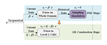
Like [6], we consider the privacy protection problem of SC worker locations in the SAT mode. Fig. 2 describes our proposed system framework that consists of four parts: CSP, SC-server, requesters and workers. Workers send their real location information to CSP. As a trusted third party, CSP collects locations reported by workers, and construct PSD with noises. Requesters submits tasks and exposed location information to SC-Server. After receiving a task request, the untrusted SC-server determines by querying the PSD and initiates a geocast communication process.
The SC-server is assumed to be semi-honest and intentionally deduces sensitive information of locations from the PSD. Under mutually-agreed upon rules with workers for data disclosure, CSP exposes PSD release (without identities and locations) to SC-servers and contacts workers in the . CSP plays mainly the role of communications, and computations to generate are carried out at the SC-server part. Possible disclosure of worker location and identity after her consent to the task is outside our scope.

To be specific, our work focuses on the design of PSD using historical data learning at CSP part. Based on historical locations, we adopt linear regression method to make prediction and simulate the real-time distribution of locations at the level-1 grid, which yields the partition together with adaptive grids (AG) method. Then CSP publishes the PSD with noisy real-time counts. Fig. 3 describes the procedure of building PSD with learning. See Section 4.2 for details.
As shown in Fig. 2, the whole scheme consists of the following steps.
-
Step 0:
Workers report their real locations to the CSP, which will be divided into real-time and historical data.
-
Step 1:
A requester sends task to SC-server.
-
Step 2:
SC-server queries the PSD with the CSP.
-
Step 3:
According to the given privacy budget , CSP partitions the data domain by learning historical locations reported by workers and imports noisy real-time counts into the generated grids to update the PSD for answering to SC-server.
-
Step 4:
SC-server determines and initiates a geocast communication process in two ways (infrastructure-based or infrastructure-less mode) as in [6].
-
Step 5:
If a worker in accepts the task, she sends a consent message to the SC-server (or the requester) for confirming her availability.
The above scheme is mainly designed for a single-task assignment system model in dynamic scenarios where for each real-time task request, the CSP collects properly the latest real-time location data of workers and updates the PSD with newly confirmed historical data, and only a worker is required to complete the task. If worker locations change rapidly, our scheme allows fixing the grid structure and updating only real-time counting in cells, which is assigned the same privacy budget. This is a significant advantage of our scheme, in particular on running time, see Section 6.4.
In the static scenario, SC-server deploys a fixed PSD in a period to release , and Steps 0, 2 and 3 can be skipped. In the case of multiple tasks, our system model is still valid under the assumption that the task assignments do not interfere with each other.
4.2 Building PSD with Learning
The first stage in our framework consists of building a PSD (at the CSP part), which determines the accuracy of released data and also affects performance metrics. Here we improve the extended Adaptive Grid method (AG) developed in [6] with historical locations learning. Table I summarizes the notations used in our description.
| Symbol | Definition |
|---|---|
| Total privacy budget | |
| Total count of workers by prediction | |
| Predicted worker count in first-level cell | |
| The first level grid granularity | |
| Second-level partitioning granularity at cell | |
| Budget allocation parameter for prediction, | |
| Parameter for domain partitioning in [6], |
The work flow of our improved AG is shown in Fig. 3. Compared to the extended AG proposed in [6], our PSD construction takes advantage of historical data learning. The detailed procedure is given as follows.
Firstly (Step ① in Fig. 3, level-1 partition), as before, at the first level, AG creates a fixed-size grid over the data domain with the level-1 granularity chosen as
| (5) |
where is the noisy total number of locations computed by adding random Laplace noise with scale , is used here just as a parameter for partitioning (privacy cost is a small fraction of the total budget ) and as in [6].
Secondly (Steps ②-③ in Fig. 3, prediction with historical data learning), historical data (without noise) are imported into the level-1 grid to make prediction of each cell’s count. The historical data divided by periods is denoted by . AG issues count queries in all level-1 cells for each , denoted by . For each cell , the linear regression on yields , a locally predicted count of the real-time locations in cell . Then, the probability distribution is evaluated with fractions of predicted total locations.
Next (Steps ④-⑤ in Fig. 3, simulation and level-2 partition), according to the probability distribution of locations on level-1 cells (as index nodes) predicted above, randomly generate points (independent and identically distributed, i.i.d.) to simulate the real-time distribution. Then level-2 granularity for each level-1 cell is chosen as
| (6) |
where denotes the point count on cell by sampling simulation and is selected as in [6] and is still a parameter with = 0.5 but not privacy budget.
Afterwards (Step ⑥ in Fig. 3, sanitized countings), real-time locations are imported into the adaptive grids generated above, and the location count in each cell are added by Laplace noise with scale . We mention that each noisy count is set zero immediately if negative. Then the PSD is completed as is processed in Fig. 3.
Indeed, we can use only real-time data even in the simulation for level-2 partition which costs no privacy budget. However, location distribution sometimes changes rapidly and irregularly while historical data learning provides the overall trend of distribution theoretically. Such a scheme using historical data allows us to fix grid structure and update only noisy real-time count in each cell for quick release of tasks while workers move rapidly.

4.3 Geocast Region Construction
In this section, we mainly introduce some new strategies for constructing . We investigate some techniques across local cell selections to fuse those cells with negative noisy counts and develop a quality scoring function involving the area of cells instead of utility function for cell selections.
Currently we consider just the static case for task locations. The probability of a worker accepting a task is only related to the worker-task distance. We refer to the mean contribution distance (MCD) proposed in [29], where the MCD is computed as
| (7) |
where is the location of worker , and the locations of its contributions. Following [30], we regard of as maximum travel distance (MTD) that is the maximum distance a worker accept to travel to perform a task.
In contrast to the utility function proposed in [6], we introduce a quality scoring function that considers noisy worker count and the cell-task distance as well as cell’s area. For adding each neighboring cell to , the score of cell in the candidate heap for task is defined as:
| (8) |
where represents the number of noisy workers in candidate cell , the area of cell and the cell-task distance computed by the average distance between the task and four corners of cell . It is reasonable that the higher density of workers in cell or the shorter the cell-task distance , the higher score . The functions and are (positive and) monotonic on and , respectively, and linear mappings to some interval . Such functions are designed to control the influence of varying the factors, area and distance.
Our algorithm to construct is shown in Algorithm 1.
In Line 2, in order to improve the compactness of the , we set a restriction by Local Maximum Geocast Region (LGR) centered at task during cell selection and the radius computation of is presented in Section 5.2. In Line 11, we add a termination condition for cyclic program in the case that all candidate cells include non-positive (and noisy) count of workers, which will be discussed in detail in Section 5.3.
In Lines 4 and 14, we calculate the utility value of some cell by, the utility function naturally defined in [6],
| (9) |
Here, denotes the noisy count of workers in cell , represents the average task acceptance probability of each worker in cell . All workers in the same cell are regarded to have the same value. Then gives the probability that no workers in are willing to perform the task . The practical meaning of is the probability that at least one worker in cell is willing to finish task . All possible candidate workers for each task are limited in the maximal distance from task . The value is assumed to decrease linearly with distance and defined as
| (10) |
where represents the average distance between the task and the four corners of the cell , and is defined as the maximum task acceptance rate of workers. Once the worker-task distance reaches , the vanishes.
In Line 15, after adding to , we should update the utility by
| (11) |
Once reaches the expected utility , it returns directly. Otherwise, we continue to select a new neighboring cell which ensures that the is a continuous region. The significant effect of using quality scoring function is shown as in Fig. 4, see Section 5.1 for details.


4.4 Performance Metrics
Adding noise to protect worker locations in SC will inevitably reduce the validity of worker-task matching and efficiency of task assignment.
To be specific, a notified region with a (noisy) positive count may contain no workers. Some workers may be notified of the task with long distance while nearer workers have no tasks. Moreover, some redundant messages for notification increase overhead. In order to evaluate the performance of the framework, we concentrate on the following performance metrics proposed in [6].
-
(1)
Assignment Success Rate (ASR). As usual, ASR measures the ratio of tasks assigned successfully to the total number of task requests. The challenge for us is to ensure that ASR reaches the threshold in the average sense of many task assignments.
-
(2)
Worker Travel Distance (WTD). Long distance will inevitably affect the efficiency of task execution. The goal is to keep the actual worker-task distance as small as possible on average.
-
(3)
Average Number of Notified Workers (ANW). ANW affects both the communication overhead of the and the computation overhead of the matching algorithm. Its goal is to inform as few workers as possible without compromise on the ASR.
-
(4)
Average Hop Count Required for Geocast (HOP). In practice, task notifications to workers in are sent by hop-by-hop wireless communication. HOP means the hop count required to disseminate the task request to all workers in given region. We approximate HOP as diameter of the divided by the diameter of the communication range ( meters for WiFi).
-
(5)
Digital Compactness Measurement (DCM). Based on the assumption that the communication cost is proportional to the minimum bounding circle that covers , the ratio of the area to the area of the smallest circumscribing circle, denoted by DCM, is adopted to measure the compactness of . Generally, the high compactness of the is helpful in reducing communication costs. The challenge is to make DCM as close to 1 as possible.
5 Selection Strategies and Privacy Analysis
In this section, we introduce three practical cell selection strategies involved in the R-HT scheme in detail and give privacy analysis of the whole system framework.
5.1 Cell Selection by Quality Scoring
The goal of our scheme is firstly to reduce communication cost and improve the success rate of task assignment when constructing for a single task, which requires suitable strategy of cell selection. The utility function involving worker count and worker-task distance is usually used in previous schemes, such as G-GR. It selects a neighboring cell with the maximum utility in each step, which would makes the number of cells in as small as possible. Indeed, in the two-level grids structure, the difference of worker counts between cells is often small. For the neighboring level-2 cells, cell-task distances are close to each other, but the gaps on area are often very large, even dozens of times, while the utility function ignores the influence of the area. This will inevitably increase communication overhead. For this reason, we consider to harness quality scoring function derived from the exponential mechanism which comprehensively takes all of the three factors into account. We compare the effects of utility function and quality scoring on Yelp (Ye.) dataset, see Fig. 4. Both functions and are assigned as linear mappings to based on series of experiments. For more detailed experimental settings, see Section 6.1.
From the perspective of the quality scoring function versus the utility function, experimental results on real-time data show that the G-GS (using scoring) performs a little better than G-GR (using utility), and G-GS improves , , and on WTD, HOP, ANW and DCM, respectively. This has no increase on ASR, while both of the new schemes with historical data learning, G-HS and G-HU, have increase on ASR. The G-HS (using scoring) maintains the above advantages on the above four indexes, since G-GS and G-HS prefer small cells with high worker density. The above analysis reflects fully the advantages of quality scoring function strategy.
From the perspective of using historical data, it can be seen that G-HS and G-HU (with historical data) have higher ASR than , while most of results for G-GS and G-GU failed to meet . Indeed, some negative noises in level-2 cells reduce worker count to be less than 0 and the cells’ utility is usually set zero. In the construction stage, the cells with a high noisy count are preferred which makes that more cells with positive noise are selected into in probability and more positive virtual counts generate. Then the noisy utility of is generally higher than the real value. In other words, when the noisy reaches , sometimes the real may not. As for using historical data learning, the zero allocation of privacy budget in the level-2 partition makes the (counting) noise scale smaller, the deviation between noisy and real is smaller so that the (real) ASR increases naturally. By the comparison of G-HS_Ad (adjusting of G-HS point by point to make its ASR value close to that of G-GS) to G-GS, we find out that in the average sense the indexes, WTD, HOP, ANW and DCM using historical data are , , and better than those using real data, respectively.
5.2 Local Maximum Geocast Reigon
In order to improve the compactness of , we set a local maximum geocast radius by adaptive search when selecting cells. We consider all cells in Local Maximum Geocast Reigon (LGR) as a whole, calculate the average distance by weighting with the absolute value of noisy counts, and then estimate the utility of the area. The initial value of is the average distance from the task to the four corners of the cell covering the task, and it increases with the fixed step that equals half the width of the smallest cell in whole domain, until the approximate utility reaches . The algorithm for finding is shown in Algorithm 2.
We consider the effect of the trick by performing experiments on NYTaxi (Ta.) dataset, and the results are shown in Fig. 5.
From the comparisons of R-GS (with LGR trick) to G-GS, and R-HS (with LGR trick) to G-HS, respectively, we observe that applying does not obviously weaken the ASR. However, it performs effectively on other metrics, especially improves and (WTD), and (HOP), and (ANW), and (DCM), respectively, with the privacy budget of 1.0. After adjusting the to make the ASR of the four schemes approximately the same, the advantage of the R-HS is more prominent on the metrics. Compared with R-GS, R-HS improves , , and , respectively. In Section 6, a series of experiments will demonstrate the effects of our budget allocation strategy with partition simulation by historical data learning from multiple perspectives.
5.3 Break for Nonpositive Neighbor Case
As is mentioned in Section 5.1, adding noise generates some negative cells (where noisy count of workers is negative) which have no contributions on utility. For this, we set a ”Break” strategy. Except for the initial cell that covers task , when the alternative neighboring cells are all non-positive, the current are returned directly. We focus on the ”Break” strategy with experiments on the Gowalla (Go.) dataset, and the results are given in Fig. 6.
It can be seen from the CELL index (number of cells in ) that with application of ”Break” strategy the CELL is reduced by without causing a significant decrease in ASR. This indicates that the real utility contribution of so-called negative cell is relatively small in the average sense. Besides, the WTD and HOP are reduced by about and , respectively.
5.4 Privacy Analysis
In this section, we focus on the analysis of privacy budget allocation and protection in the whole system framework. The budget allocation is detailed as in Fig. 7.
Firstly, due to the nature of unbounded DP, we have to allocate a small fraction of privacy budget to noisy count of the total locations in the domain for level-1 partition.
Secondly, for level-2 partition we employ historical data learning to make sampling simulation of current distribution. Usually the prediction by learning of historical locations has correlation of real-time data no matter whether noises are added on original data. For this, we use the probability distribution determined by the predicted proportion on counts to perform random sampling (i.i.d.), which achieves a nice simulation of current distribution without privacy costs. Such a method helps us learn the overall distribution of locations in the statistical sense. Based on the sampled points (only used for local counting) generated independently, any adversary can not guess which (level-1) cell a specific worker is currently located in. Moreover, the level-2 partition costs no privacy budget.


Thirdly, in the construction stage, real-time data is imported into the partitioned grid, and Laplace noise of main privacy budget is added to each level-2 cell in parallel.
Finally, the involved learning on historical data, “Break” strategy and operations suit the characteristics of post-processing (Theorem 3), and the whole system scheme satisfies -DP protection.
6 Performance Evaluation
In this section, we mainly present an experimental evaluation of our R-HT scheme. In particular, we compare R-HT with previous schemes, like G-GR.
6.1 Experimental Methodology
Experimental comparison. Historical data learning technique has been proved to provide relatively high predictive accuracy [21, 20]. In order to verify the system quality of the proposed R-HT scheme, we carry out a series of experiments to compare it with the GDY [4], G-GR [6] and G-GS. Indeed, the G-GS scheme is modified from G-GR, where the utility rule is replaced by quality scoring for cell selections.
These privacy frameworks are achieved based on the notion of unbounded DP. Then the sensitivity of workers’ count in each grid (or region) is , that is, while the maximum increase or decrease is 1 for the total number of workers, such a change may occur in any cell [28]. Compared with unbounded DP, the sensitivity in bounded DP case is , and the increase of noise scale would significantly affect the success rate of task assignment.
Selection of Datasets. We use three real datasets: NYTaxi (NYC’s Taxi Trip Data), Gowalla and Yelp.
NYTaxi is a New York taxi location dataset. We extract taxi pickup positions in New York City during 21 days, May 1 to 21, 2013. The first 20 days are used as historical data, and 27,165 positions on May 21 as real-time data. Each pickup position is modeled as a worker position in spatial crowdsourcing (SC). Since most of the taxi pickup positions are distributed on the city’s main roads, in order to better simulate the actual positions of workers, we randomly and uniformly blur each position into a circle centered at the current position and with the radius (Blur Radius, BR) of 80 meters.
Gowalla is a social network check-in dataset. We extract the check-in locations for 42 days from September 5 to October 16, 2010. Due to the large geographic span of data, we reduce the geographical distance by a ratio of . Every two days are regarded as a period, and the last period includes 6,736 location points for real-time data. Each restaurant location is modeled as a worker position in SC, and the BR is 250 meters.
Yelp corresponds to some data of the Phoenix area of Arizona. We take location data from March 2014 to August 2017 and assign 2 months as a period. The last period with 17,730 locations was used as real-time data. We also model the location of each restaurant as a worker position in SC, BR is 600 meters.
| Name |
|
|
MTD/m | Tasks | ||||
|---|---|---|---|---|---|---|---|---|
| NYTaxi (Ta.) | 841080 | 27165 | 300 | 2000 | ||||
| Gowalla (Go.) | 133771 | 6736 | 1200 | |||||
| Yelp (Ye.) | 363330 | 17730 | 3000 |
We can set scenes for the above three datasets separately. NYTaxi dataset can be regarded as a taxi ordering scene in the downtown. The maximum distance for taxi drivers to perform orders is 500 m. is 300 m, usually equal to of which is determined by Eq. (7). For Gowalla, we can consider a takeaway booking scenario in which the maximum order distance is 2 km, and then the is 1.2 km. Yelp can be a model of an auto repair scenario. The maximum order distance is 5 km and is 3 km. Besides, 2,000 positions are randomly and uniformly selected from the worker positions as task points. The relevant parameters of the datasets are shown in Table II.
In our experimental settings, privacy budget , expected utility , and maximum task acceptance probability . The default values for , and are set to 0.5, 0.9 and 0.1, respectively. The functions and involved in quality scoring function are linear mappings to from the interval between minimum and maximum areas of cells, and between the half length of diagonal line in the minimal cell and , respectively.
The utility loss caused by DP can be seen more intuitively by performing a non-privacy scheme, which constructs by selecting workers closest to the task one by one within the reigon. The HOP value of is defined as the distance between the two farthest workers. As for GDY and G-GR, in order to avoid the influence of the randomness of noise on partitioning, we carry out the whole process 50 times to obtain 50 groups of results and get their average values. For R-HT, the simulation process of grids partition is independently executed 10 times, which results in 10 groups of partitioned grids. The real-time location counting noise in each level-2 cell is randomly added for 20 times separately, and then a total of 200 PSD snapshots are generated. For all schemes, 2000 single-task assignments are performed on each map, regardless of possible conflicts between task assignments, so as to obtain stable results of performance evaluation of each scheme under this scenario (single worker requested for single task). Next, we investigate the effects of varying privacy budget, and expected utility, respectively, and also evaluate -based heuristics and the running time of the schemes for feasibility.


6.2 Task Allocation Evaluation
In this section, we evaluate the performance of R-HT and some closely related schemes on three datasets by varying parameters, including privacy budget , maximal acceptance rate , and expected utility . Performance is measured by the five main metrics presented in Section 4.4.
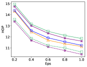
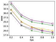
6.2.1 Effect of Varying Privacy Budget
We firstly investigate the impact of varying the privacy budget while keeping the other parameters at their defaults, see Fig. 8. With the default =0.9, almost all ASR values of R-HT reach the threshold, while G-GR fails in most cases. As for WTD, HOP and DCM, R-HT is , and better than G-GR on average, and has a maximum increase of , and , respectively. This demonstrates that R-HT ensures basically that the task acceptance probability reaches , and it behaves better than G-GR in other metrics. The reason is that the use of historical data significantly reduces the noise added to the grid partition and real-data publication. Smaller noise makes the adaptively generated grids more suitable and yields that cell selections are inclined to be of higher density and closer distance. Besides, the ASR of R-HT in NYTaxi is relatively low. In fact, the location distribution is very concentrative on roads, which yields many smaller cells locally. is set small, which makes decreasing sharply with the increase of distance. Then the larger count of cells needed for results in more virtual locations, and the real ASR will be lower when noisy ASR reaches .
By adjusting to R-HT and GDY to make the ASR of all schemes almost the same, the advantage of R-HT_Ad (R-HT with adjusted ) is more obvious. Compared with G-GR, the average decrease of HOP for R-HT_Ad and G-GS is and , respectively. R-HT_Ad behaves perfect on WTD, with an average reduction of , while it reduced the notified workers (ANW) by compared with G-GR. In addition, we observe that for the change of DCM, GDY makes the best performance. Indeed, GDY has the coarsest partitioning granularity, which results in the smallest number of selected cells, even the cell covering task is enough for . The DCM of R-HT_Ad is higher than that of G-GR because of applying strategy.
To sum up, within the wide range of privacy budget, R-HT can basically meet , effectively reduce the actual system cost for task assignments, and also improve the compactness of for effectively saving communication costs, which improves system operation efficiency comprehensively.
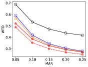
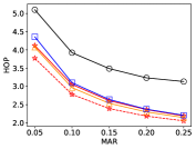
6.2.2 Effect of Varying MAR
We observe the metrics for R-HT by changing and make some comparisons, see Fig. 9. The experimental results show that the increase of reduces the HOP and WTD soon, because it increases AR of each worker and fewer workers nearby are needed for achieving the requirements of . Further, with the increase of , the decrease of cell count in is more obvious than the impact of changing . Except for a few points, the ASR of R-HT meets , while the ASR of G-GR fails on nearly a half of points. Compared with the G-GR, the average improvement of R-HT_Ad on the WTD, HOP, ANW and DCM are , , and , respectively.
6.2.3 Effect of Varying
We observe the influence of changing on the metrics of R-HT and other schemes. Obviously, when increases, the area increases, and so do both WTD and HOP. The results show that for varied , each ASR of R-HT meets the threshold and the WTD and HOP are always smaller than those of G-GR, respectively. With the increase of , the gaps are wider due to more cells necessarily selected. When equals 0.9, the gaps between R-HT_Ad and G-GR on WTD, HOP, ANW and DCM are up to , , and , respectively.


In conclusion for Sections 6.2.1 to 6.2.3, according to the ASR results above, the R-HT basically reaches under various parameter settings. In most cases, the G-GR fails to reach , as is mentioned in Section 7.2.1 of [6]. Therefore, G-GR does not address the challenge of achieving a high success rate for the task assignment. To be specific, a total of 42 groups of ASR values are compared in different settings of parameters , and on three datasets. Among them, 19 points of G-GR reach , accounting for , while 38 points of R-HT accounting for , twice as much as G-GR. We find out that the compliance rates of ASR on Yelp, Gowalla and NYTaxi, G-GR is , and , while R-HT , and , respectively. Both of the two schemes have some gaps on compliance rate in NYTaxi due to the extremely concentrative distribution of locations as is mentioned above.


6.3 Evaluation of LGR-Based Heuristics
Experimental results illustrate that strategy improves the schemes as is mentioned in Section 5.2. However, we find that the local radius computed by Algorithm 2 is sometimes too large. Indeed, in the construction stage, the proportion that the whole cells are still not enough for reaching , for adopting , and is very low. We perform the R-HT schemes with 0.9 and 0.88, respectively, to compare with the improved hybrid scheme of the G-GR. The experimental results on Gowalla are shown in Fig. 11.
When local radius is reduced, the ASR of R-HT decreases naturally. Indeed, with the reduction of , there are more tasks whose ASR can not achieve . In the case of , most ASR values for Gowalla can still reach , while the adoption of the G-GR_hybrid scheme does not improve obviously the ASR of G-GR. R-HT has a clear advantage in WTD, smaller than G-GR_hybrid on average. As for HOP, although the two schemes are entangled to each other, R-HT still leads overall. On the ANW, R-HT is a bit higher due to the higher ASR. Further, On DCM R-HT gradually loses the advantage, which is mainly related to the utility function of G-GR_hybrid, defined by
| (12) |
where , represents the task acceptance probability of cell , and is the DCM of with cell included. As increases, the DCM weight in the utility function becomes larger. When is equal to 1.0, the utility function only depends on DCM.
By comparing with non-privacy algorithm, we can observe that non-privacy has obvious advantages in WTD and HOP because it has no grids. On ANW, we can see that 0.88R-HT, G-GR and G-GR_hybrid are close to the non-privacy scheme when equals 1.0, which indicates that the three schemes behave well on reducing ANW, and among them the ASR of 0.88R-HT is the highest at this point.
Besides, we mention that To et al. [6] proposed a partial cell selection based on G-GR to deal with the ASR overflow problem when adding the last cell to , which reduces system overhead to some extent. However, due to the severe challenge that the actual ASR fails to reach , the partial cell selection undoubtedly aggravates this trouble, which is demonstrated by our various experiments. Therefore, the partial cell strategy in R-HT is not skipped in this paper.
6.4 Test on Running Time
In real life, despite the success rate of task assignment and communication cost, the time costs from task request to GR release is also very important. We divided the entire assignment process of a single task into two major stages. The first stage is the domain partitioning (stage A), which includes the partitioning and adding noise to the number of real-time workers. Due to using historical data, this stage can be divided into the following two parts: Partitioning with noisy historical data (Stage A1); Then, updating real-time data and adding noise to the count of workers in level-2 cells (Stage A2). The second stage is the construction stage (Stage B).
We consider the following three comparisons in terms of time consuming: First, the entire process (A+B), which means the running time of the entire algorithm; Second, updating real-time count in each cell and constructing (A2+B) with fixed grids, which is applicable to scenarios where the real-time data changes greatly in a period and we need only to upload real-time data for updating ; Third, constructing after updating real-time data (B).
We use Python 2.7 on Windows 10 (2.4 GHZ Intel i5 CPU, 8G RAM) to run 2,000 tasks on 3 datasets, and calculate each time cost by taking the average of 10 cycles, see Table III.
| Stage |
|
|
|
||||||||||||
|---|---|---|---|---|---|---|---|---|---|---|---|---|---|---|---|
| R-HT | G-GR | R-HT | G-GR | R-HT | G-GR | ||||||||||
| B | 20.4 ms | 0.5 ms | 9.8 ms | 0.5 ms | 16.9 ms | 0.6 ms | |||||||||
| A2+B | 21.3 ms | 10.1 ms | 17.5 ms | ||||||||||||
| A+B | 1.60 s | 62 ms | 0.56 s | 22 ms | 2.83 s | 0.1 s | |||||||||
It can be seen in the table that in stage B, R-HT takes a relatively long time, because R-HT needs to calculate , cell’s utility and cell’s score. For Stage A2+B, compared with stage B, updating data and adding noise only takes a very small period of time (less than 1 ms), and there is no data updates in G-GR after partitioning. In Stage A+B, The time consumption in partitioning is far greater than that in construction, mainly due to the fact that the process of historical data prediction costs much time in R-HT.
However, our scheme is very suitable for the case that workers move rapidly, as is mentioned in Section 4.1. Fix the grids and update real-time locations. This saves much on running time (A2+B) compared with G-GR on A+B.
In a word, the running time of a single task on the three datasets is within 3 seconds, which forms an approximate direct proportion with the total count of real-time data, which guarantees the timeliness and practicability of task release in real life.
7 Conclusion
In this paper, we proposed a location protection model for worker dataset in SC based on DP, which ensures that the privacy of worker locations is not disclosed at the task assignment stage. As far as we know, we are the first to introduce historical data learning and sampling simulation into domain partitioning and then we achieved efficient allocation of privacy budget. This significantly reduces scales of random noises and enables the real ASR to reach the expected utility threshold stably. Moreover, We introduced several optimization techniques for constructing , particularly the newly designed quality scoring function. Our experimental results on real data demonstrated that the proposed R-HT scheme reduces the system overhead, and the time cost is practical.
Currently, we analyze a single-task (single-worker only) framework for privacy protection of worker locations based on historical data learning. If there is only real-time data, data segmentation (one part for domain partitioning and the other for construction) can achieve parallel composition of privacy budget, which will be discussed in a forthcoming paper. As future work, we aim to extend the privacy framework for the scenario of multi-task parallel assignments in SC and explore new cell selection strategies.
Acknowledgments
The authors thank Professor Chi Zhang for his excellent comments which greatly helped us to improve this paper.
References
- [1] H. To and C. Shahabi, Location Privacy in Spatial Crowdsourcing. Cham: Springer, 2018.
- [2] Y. Tong, Z. Zhou, Y. Zeng, L. Chen, and C. Shahabi, “Spatial crowdsourcing: A survey,” The VLDB Journal, vol. 29, no. 1, pp. 217–250, 2020.
- [3] Y. Xiao, L. Xiong, and C. Yuan, “Differentially private data release through multidimensional partitioning,” in Workshop on Secure Data Management. Springer, 2010, pp. 150–168.
- [4] W. Qardaji, W. Yang, and N. Li, “Differentially private grids for geospatial data,” in 2013 IEEE 29th International Conference on Data Engineering (ICDE), 2013, pp. 757–768.
- [5] H. To, G. Ghinita, and C. Shahabi, “A framework for protecting worker location privacy in spatial crowdsourcing,” Proceedings of the VLDB Endowment, vol. 7, no. 10, pp. 919–930, 2014.
- [6] H. To, G. Ghinita, L. Fan, and C. Shahabi, “Differentially private location protection for worker datasets in spatial crowdsourcing,” IEEE Transactions on Mobile Computing, vol. 16, no. 4, pp. 934–949, 2017.
- [7] X. Wang, Z. Liu, X. Tian, X. Gan, Y. Guan, and X. Wang, “Incentivizing crowdsensing with location-privacy preserving,” IEEE Transactions on Wireless Communications, vol. 16, no. 10, pp. 6940–6952, 2017.
- [8] C. Yin, J. Xi, R. Sun, and J. Wang, “Location privacy protection based on differential privacy strategy for big data in industrial internet of things,” IEEE Transactions on Industrial Informatics, vol. 14, no. 8, pp. 3628–3636, 2018.
- [9] T. Zhu, G. Li, W. Zhou, and S. Y. Philip, Differential Privacy and Applications. Springer, 2017, vol. 69.
- [10] R. Shokri, G. Theodorakopoulos, C. Troncoso, J. P. Hubaux, and J. Y. Le Boudec, “Protecting location privacy: Optimal strategy against localization attacks,” in Proceedings of the 2012 ACM Conference on Computer and Communications Security, 2012, pp. 617–627.
- [11] M. E. Andrés, N. E. Bordenabe, K. Chatzikokolakis, and C. Palamidessi, “Geo-indistinguishability: Differential privacy for location-based systems,” in Proceedings of the 2013 ACM SIGSAC Conference on Computer Communications Security, 2013, pp. 901–914.
- [12] B. Liu, L. Chen, X. Zhu, Y. Zhang, C. Zhang, and W. Qiu, “Protecting location privacy in spatial crowdsourcing using encrypted data,” Advances in Database Technology-EDBT, pp. 478–481, 2017.
- [13] P. Xiong, L. Zhang, and T. Zhu, “Reward-based spatial crowdsourcing with differential privacy preservation,” Enterprise Information Systems, vol. 11, no. 10, pp. 1500–1517, 2017.
- [14] H. To, C. Shahabi, and L. Xiong, “Privacy-preserving online task assignment in spatial crowdsourcing with untrusted server,” in 2018 IEEE 34th International Conference on Data Engineering (ICDE). IEEE, 2018, pp. 833–844.
- [15] Z. Wang, X. Pang, Y. Chen, H. Shao, Q. Wang, L. Wu, H. Chen, and H. Qi, “Privacy-preserving crowd-sourced statistical data publishing with an untrusted server,” IEEE Transactions on Mobile Computing, vol. 18, no. 6, pp. 1356–1367, 2019.
- [16] J. Wei, Y. Lin, X. Yao, and J. Zhang, “Differential privacy-based location protection in spatial crowdsourcing,” IEEE Transactions on Services Computing, 2019, in press.
- [17] X. Li, Y. Wang, X. Zhang, K. Zhou, and C. Li, “A more secure spatial decompositions algorithm via indefeasible laplace noise in differential privacy,” in International Conference on Advanced Data Mining and Applications. Springer, 2018, pp. 211–223.
- [18] Y. Gong, C. Zhang, Y. Fang, and J. Sun, “Protecting location privacy for task allocation in ad hoc mobile cloud computing,” IEEE Transactions on Emerging Topics in Computing, vol. 6, no. 1, pp. 110–121, 2018.
- [19] D. Xu, Y. Wang, L. Jia, Y. Qin, and H. Dong, “Real-time road traffic state prediction based on ARIMA and Kalman filter,” Frontiers of Information Technology Electronic Engineering, vol. 18, no. 2, pp. 287–302, 2017.
- [20] R. Liu, G. Cong, B. Zheng, K. Zheng, and H. Su, “Location prediction in social networks,” in Asia-Pacific Web (APWeb) and Web-Age Information Management (WAIM) Joint International Conference on Web and Big Data. Springer, 2018, pp. 151–165.
- [21] Y. Jiang, W. He, L. Cui, and Q. Yang, “User location prediction in mobile crowdsourcing services,” in International Conference on Service-Oriented Computing. Springer, 2018, pp. 515–523.
- [22] Z. Chen, X. Kan, S. Zhang, L. Chen, Y. Xu, and H. Zhong, “Differentially private aggregated mobility data publication using moving characteristics,” arXiv preprint arXiv:1908.03715, 2019.
- [23] L. Kazemi and C. Shahabi, “Geocrowd: Enabling query answering with spatial crowdsourcing,” in Proceedings of the 20th International Conference on Advances in Geographic Information Systems, 2012, pp. 189–198.
- [24] L. Kazemi, C. Shahabi, and L. Chen, “Geotrucrowd: Trustworthy query answering with spatial crowdsourcing,” in Proceedings of the 21st ACM Sigspatial International Conference on Advances in Geographic Information Systems, 2013, pp. 314–323.
- [25] X. Zhang, Z. Yang, Y. Liu, and S. Tang, “On reliable task assignment for spatial crowdsourcing,” IEEE Transactions on Emerging Topics in Computing, vol. 7, no. 1, pp. 174–186, 2016.
- [26] C. Dwork, “Differential privacy,” in Proceedings of the 33rd International Conference on Automata, Languages and Programming - Volume Part II, 2006, pp. 1–12.
- [27] C. Dwork and A. Roth, “The algorithmic foundations of differential privacy,” Foundations and Trends® in Theoretical Computer Science, vol. 9, no. 3–4, pp. 211–407, 2014.
- [28] N. Li, M. Lyu, D. Su, and W. Yang, “Differential privacy: From theory to practice,” Synthesis Lectures on Information Security, Privacy, Trust, vol. 8, no. 4, pp. 1–138, 2016.
- [29] B. J. Hecht and D. Gergle, “On the ‘localness‘ of user-generated content,” in Proceedings of the 2010 ACM Conference on Computer Supported Cooperative Work, 2010, pp. 229–232.
- [30] M. Musthag and D. Ganesan, “Labor dynamics in a mobile micro-task market,” in Proceedings of the SIGCHI Conference on Human Factors in Computing Systems, 2013, pp. 641–650.