[1]\fnmGonglin \surYuan \equalcontThese authors contributed equally to this work.
[1]\orgdivGuangxi University, \orgnameSchool of Mathematics and Information Science, Center for Applied Mathematics of Guangxi (Guangxi University), \orgaddress\streetStreet, \cityNanning, \postcode530004, \stateGuangxi, \countryChina
2]\orgnameThai Nguyen University of Economics and Business Administration, \orgaddress\streetStreet, \stateNguyen, \countryThai
A Diagonal BFGS Update Algorithm with Inertia Acceleration Technology for Minimizations
Abstract
We integrate the diagonal quasi-Newton update approach with the enhanced BFGS formula proposed by Wei, Z., Yu, G., Yuan, G., Lian, Z. [1], incorporating extrapolation techniques and inertia acceleration technology. This method, designed specifically for non-convex constrained problems, requires that the search direction ensures sufficient descent and establishes global linear convergence. Such a design has yielded exceptionally favorable data results.
keywords:
Non-convex Unconstrained Optimization, q-linear convergence, Quasi-Newton Methods, Diagonal Quasi-Newton Updates, Inertia Algorithms.1 Introduction
Address the unrestricted optimization dilemma of reducing a continuously differentiable function , represented as:
| (1.1) |
Quasi-Newton methods belong to a category of iterative optimization algorithms that employ quasi-Newton approximations of the Hessian matrix to address the problem that defined in (1.1). The underlying principle involves forming a sequence of iterates designed to converge towards a fixed point of , achieved through the iterative refinement of an approximate Hessian matrix to expedite optimization procedures with at each iteration. The foundational principles of the quasi-Newton approach originated with Davidon [2], and subsequent enhancements and applications have been explored by numerous scholars [3, 4, 5]. We start with and . The iterative process is updated by generating a sequence to iteratively refine the estimation of the Hessian matrix:
| (1.2) |
In , the determination of the search direction is governed by the line search vector , and represents the determination of the is conducted via line search procedure. The meaning of represents partial gradient of at , represented as a vector of the function we are looking for:
| (1.3) |
represents the difference vector between consecutive iterates, computed as , and the variable denotes the discrepancy vector between the gradients observed at consecutive iterations, formulated as . In algorithm for approximating the Hessian matrices, the vectors and are crucial for the enhancement of the algorithm, which is realized by an update process. BFGS updating is the most widely used among those formulations, expressed as:
| (1.4) |
Computational evidence has consistently demonstrated the superior effectiveness to other quasi-Newton methods. Considerable scholarly investigations have been dedicated to exploring the convergence characteristics of the technique , particularly in a realm of convex minimization, as evidenced by studies such as [6, 7, 8, 3, 4, 5]. These formulations have demonstrated high effectiveness in practical scenarios across a diverse range of optimization problems. By incorporating the insights garnered from these studies, we refine our existing formula in (1.4), leading to enhanced convergence performance.
Drawing inspiration from Neculai Andrei’s work on diagonal Hessian matrix from a function [9], we leverage the efficacy of the update formula (1.4) and its variants. The approach discerns the components positioned along the principal diagonal of the approximative matrix which, adhering to the principles outlined in the theory from Dennis and Wolkowicz’s [10] secant updating method with minimal changes, is a key aspect to be addressed. Let us now delve into this consideration:
| (1.5) |
holds for every , an estimate of components of the matrix for at iteration . Incorporated within the algorithm, a computation of the search direction which is expressed as , specifically, for . Notably, as is both diagonal and positive definite, every element undergoes multiplication through distinct positive factors, determined by the diagonal factors , in this particular algorithm. To facilitate the use of the minimum change secant update strategy, let us consider the assumption that the diagonal matrix possesses positive definiteness. The updated matrix , defined as an outcome of the update to , can be expressed as:
| (1.6) |
where is a correction matrix that satisfies certain conditions to ensure the accuracy and stability between and . More precisely, the matrix serves as a correction to , ensuring that is positive definite and adheres to the weak orthogonal cut condition proposed by Dennis and Wolkowicz [10]:
Utilizing (1.11) and the weak WWP step size rule,
| (1.7) | ||||
| (1.8) |
Meanwhile, Wei, Z., Yu, G., Yuan, G., Lian, Z. introduced a novel formula[1]:
| (1.9) |
where and
| (1.10) |
By using (1.9), they provided a BFGS-type update,
| (1.11) |
Therefore, our attention shifts to the modified BFGS method, a formulation demonstrated to exhibit superlinear convergence, as proposed by Wei Wei, Li, and Qi [1]. They have introduced several modifications to the BFGS method incorporating the recently introduced quasi-Newton condition . Employing this property within the framework enables the establishment of its linear convergence.
This observation motivates us to combine these two derivations of and obtain a new improved formula, which simplifies the proof of convergence. In utilizing the iterative update approach, let us make the assumption that the matrix should be positive definite. So derived from the update which is defined by , expressing as a formula to approach , recognizing and are vectors. Often, in practice, from (1.2) is defined from WWP step rules [11, 12] with the selection of positive coefficients and ensuring .
Section 1 of this paper introduces the research problem and recent advancements in related studies. Section 2 explains the motivation behind this research and proposes the improved diagonal quasi-Newton algorithm, DMBFGS3, as well as the WDMBFGS3 algorithm, which incorporates extrapolation techniques. Section 3 proves the global linear convergence of both algorithms. Section 4 validates the rapid convergence and stability of the WDMBFGS3 algorithm through numerical experiments. Section 5 wraps up the findings discussed in this paper and proposes avenues for further investigation.
2 Motivation and algorithm: Optimizing Hessian with Diagonal Minimization
As previously mentioned, the matrix from (1.6) is ascertained as the result of the following questions:
| (2.1) | ||||
Then we can further modify the definitions of and ,obtain the following formula:
| (2.2) | ||||
The objective function of problem (2.2) constitutes a linear combination of minimizing the difference between and according to the principle of variation, along with minimizing the sum of the diagonal elements of . The incorporation of within the target function from (2.1) is motivated by the aim to derive a correction matrix ,
| (2.3) | ||||
where, , and The Lagrangian corresponding to problem (2.3) can be said to be:
| (2.4) |
that represents the lagrangian coefficient.Solutions pursued to this problem (2.3) correspond to a fixed point of the Lagrangian. Consequently, we take the partial derivative of (2.4) for , so we can obtain:
| (2.5) |
By transferring items, we can obtain:
| (2.6) |
To determine , we use the constraint in (2.3) and substitute (2.6) into it, which gives:
| (2.7) |
where . By utilizing (2.7) in (2.6), we can express the diagonal elements of as follows:
| (2.8) |
where is the serves as the Hessian matrix. This diagonal correction matrix can be articulated as
| (2.9) |
Then we have the following equation:
| (2.10) |
i.e., on components,
| (2.11) |
The vector is then ubsequently performed as:
| (2.12) |
where is the gradient at the new point, and is the search direction. It is essential to note that, in order to prevent the update matrix from degenerating or becoming an indefinite matrix , it’s necessary that holds for all . If , then ; otherwise, , where denotes a minor positive constant.
In practical scenarios, the pursuit of iterative algorithms with rapid convergence rates remains a consistent focus of research [13, 14, 15, 16, 17, 18]. Among these, the inertial extrapolation method has gained significant attention as an acceleration approach [19, 20]. These methods rely on iterative schemes where each subsequent term is derived from the preceding two terms. This concept originated from Polyak’s seminal work [21] and is rooted when dealing with a dissipative dynamical system that is second-order in time, we employ an implicit discretization technique.This arrangement is delineated by the subsequent differential equation:
| (2.13) |
Let and be a differentiable function.
The discretization of arrangement (2.13) enables the determination of the subsequent term
given the previous terms and using an iterative scheme. This discretization process is crucial in the development of inertial extrapolation methods, which aim to enhance the convergence rate of iterative algorithms. By leveraging information from the two preceding terms, these methods efficiently approach the desired solution. The specific form of the discretization and the iterative scheme employed depend on the particular inertial extrapolation method in use. However, the underlying principle remains the same: harnessing the momentum generated by previous iterations to expedite the convergence process.
Arrangement (2.13) is discretized in such a manner that, possessing the terms and , the subsequent term can be ascertained utilizing
| (2.14) |
where is the pace magnitude. Equation (2.14) begets the ensuing iterative plan:
| (2.15) |
where , , and is denoted as the inertial extrapolation term aimed at accelerating the convergence of the series produced from Equation 2.15.
Recently, a plethora of algorithms rooted in the inertial acceleration technique, initially proposed by Alvarez [22], have emerged to tackle a diverse array of optimization and engineering challenges. Notably, the fusion of inertial acceleration with finely crafted search direction strategies, as advocated by Sun and Liu [23], has garnered significant attention.Building upon this groundwork, [24] has made significant contributions for addressing nonlinear monotone equations. The convergence being confined and meeting certain descent conditions:
| (2.16) |
The inertial extrapolation step magnitude is selected as:
| (2.17) |
In this case, where , the stipulation in (2.16) is satisfied automatically.As is commonly understood, the aforementioned condition is stronger than the one typically used:
| (2.18) |
There are some algorithms obtained through inertial extrapolation techniques [25, 20, 26, 19], it becomes apparent that by setting
| (2.19) |
Considering these two algorithms, we can observe that with increasing iterations, the discrepancy between and becomes smaller and smaller. Therefore, the step size determined by (2.16) will achieve better convergence compared to (2.18).
From the preceding process, we proposed the following algorithm:
Based on extrapolation techniques, we have accelerated the convergence speed of the DMBFGS3 algorithm using extrapolation techniques. The resulting algorithm is as follows:
Remark
-
•
We introduce a novel approach based on the theory of minimal alterations in secant updates proposed by Dennis and Wolkowicz [10]. In our method, we enforce the condition that the updating matrices are diagonal, which serves as the approximation to the Hessian. We have improved the search strategy for and achieved linear convergence for the entire algorithm.
-
•
Our experimental results demonstrate that the algorithm proposed by combining these two methods is more efficient and robust compared to other benchmark algorithms.
3 CONVERGENCE OF ALGORITHMS
The subsequent assumptions are necessary for this article:
-
•
The function exhibits continuous differentiability over the set , with for all , where is a non-negative constant.
-
•
The set of level points, denoted as , is enclosed within the set .
-
•
Indicating that , and the function is convex, such that for all .
-
•
There exists which represents the solution to the minimization problem stated in (1.1).
Lemma 1.
Assuming that for each , and the function meets the required conditions, consider the sequences of diagonal matrices and are generated by (2.9) and (2.10)
Assuming the existence of constants and satisfying for every , where is the diagonal element of the matrix , it follows that the sequences and remain finite for each .
Proof.
By Equation 2.9 and Equation 2.10, since is a diagonal matrix, we can derive the iterative formula for its diagonal elements (2.11), and . Because of use Equation 2.11 we can have:
| (3.1) | ||||
Since , it implies the existence of , whereby , . Therefore,
Since , using of assumptions , we can deduce that
Set
for each , use of , we can deduce that
The diagonal matrix sequence is bounded , beacuse of Equation 1.6 , the sequence is bounded, too. ∎
Lemma 2.
Suppose that the required elements are produced by the algorithm DMBFGS3. Then for any , the function value can be represented as:
| (3.2) |
where .
Lemma 3.
Suppose that the elements consists of algorithm DMBFGS3 and that is continuous on . So
| (3.3) |
Proof.
We derive the following equation through the expansion of Taylor’s series:
and
where and From the definition of and Lemma 2, we get
and
Hence,
Therefore, Lemma 3 holds, and is definitely bounded, we can set the boundary of this sequence as . ∎
Lemma 4.
Let be produced by the DMBFGS3 algorithm. There exists a sequence of positive numbers and a sufficiently large positive number , thereby for iterations , it holds that
| (3.4) | ||||
Proof.
From Equation (1.6), for a given , we have . Hence,
| (3.5) | ||||
Since ,we have
| (3.6) | ||||
Since we have:
| (3.7) | ||||
Since , exists , thereby , . Therefore, . Hence,
| (3.8) |
But,
Hence
Therefore,
Since , exists thereby . Therefore, . Hence,
But,
Hence
So, we have
| (3.9) |
But, from Lemma 1,
Using (3.7) and Lemma 1, it deduces that:
| (3.10) |
Examining Equation 3.6, we find:
| (3.11) | ||||
Also, considering the terms in (3.8) and (3.9), we get:
| (3.12) |
From (3.5), using (3.6), (3.10), and (3.11), we have:
where , i.e., (1.11) fulfills the property of bounded degradation.
∎
In particular, the sequences is bounded. The ensuing proposition establishes the quadratic-linear convergence of the DMFBGS3 technique. The validation relies on the characteristic of restricted deterioration as delineated in Lemma 2 (consult [27] for comprehensive validation).
Theorem 1.
Presume that the modification equation (2.10) adheres to the confined degradation attribute. Additionally, assume the existence of the affirmative constants and ,we have:
Next, the succession produced by the technique DMBFGS3 is properly delineated, and converges q-linearly to .
Theorem 2.
Suppose and are produced by Algorithm Algorithm 2. Assuming , then according to Assumptions, it is true that
Proof.
| (3.13) | ||||
Since the sequence is convergent, there exists an such that . Similarly, we can deduce that .Through Theorem 1, we can obtain , Through (3.13), we can obtain:
| (3.14) |
So that
| (3.15) |
∎
The convergence of the algorithm DMBFGS3 is ensured, and the sequence exhibits q-linear convergence towards ., while the sequence also converges efficiently.
4 Data Analysis
All code was written and executed on a personal computer equipped with an Intel 13th Gen Intel Core(TM) i5-13490F processor (running at a speed of 2.50 GHz). The machine has 32.0 GB of RAM (31.8 GB usable). MATLAB r2021b was used for coding and execution.
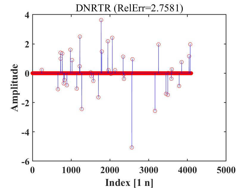
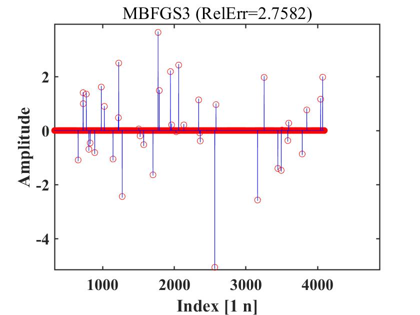
To support the theoretical results, this paper compares two classic quasi-Newton optimization algorithms: DNRTR [9] and MBFGS3 [1]. MBFGS3 is an enhanced quasi-Newton algorithm with a modified term added to , while DNRTR is a diagonal quasi-Newton update method for unconstrained optimization.
4.1 CS problems
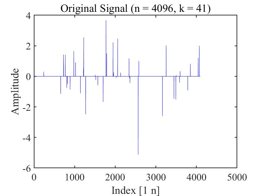
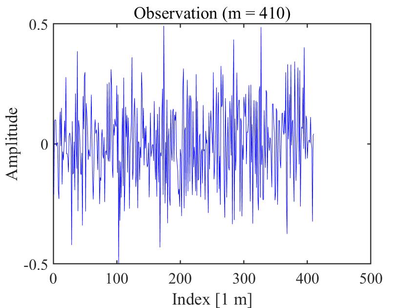
Candes et al. [28] and Donoho [29] have highlighted significant advancements in the field of Compressive Sensing (CS) in recent years.Compressive Sensing (CS) is a theoretical framework for efficiently acquiring and reconstructing sparse or approximately sparse signals. In this theory, sparsity implies that a signal can be described using a relatively small number of non-zero components, such as the coefficient vector in an appropriate basis or transform. In essence, Compressive Sensing involves the concept of representing a large, sparse signal with a limited number of linear measurements using a matrix and then storing . The primary difficulty lies in reconstructing the original signal from the observation vector .
We applied the proposed method to the CS problem, a swiftly expanding discipline that has attracted significant interest across multiple scientific areas. We assess the quality of the reconstructed signal by calculating the relative error compared to the original signal as follows:
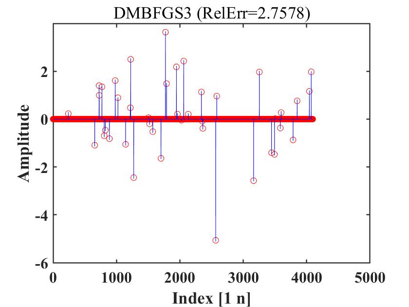
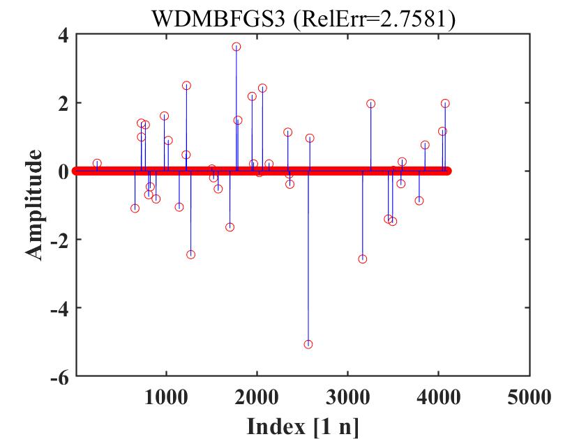
Following the method described in [30], we created random test functions by setting the signal dimension to and using the Hadamard matrix for the sampling matrix . We performed a comparison among WDMBFGS3, MBFGS3, DMBFGS3, and DNRTR using a Bernoulli matrix , with entries randomly taking values of or with equal likelihood. This setup allows us to evaluate the performance of these algorithms under the specified conditions and matrix structure. The initial point was set to .To perform a meaningful comparison of these approaches’ performance, the resulting data was analyzed in terms of relative error (RelErr).
Figure 4 to Figure 6 compare MBFGS3, DMBFGS3, DNRTR, and WDMBFGS3 in terms of function values versus reconstruction ability (Refer to Figure 4-Figure 6, which illustrate the recovered signal (red circles) compared to the original signal (blue peaks)). These figures verify the competitiveness of WDMBFGS3 compared to MBFGS3, DMBFGS3, and DNRTR based on the corresponding values. Furthermore, by examining the plots and noting the real reconstruction errors, the effectiveness and resilience of the WDMBFGS3 method in retrieving large sparse signals become evident when compared to the alternative solvers. This approach is seamless and can be efficiently addressed using the provided algorithm.
4.2 74 Unconstrained Optimization Test Problems
To compare the numerical performance between WDMBFGS3 and DMBFGS3 methods, we compared them using various techniques . This study assessedthe CPU time (CPU) , the number of function evaluations (NFG), and the iteration count (NI) of the algorithms required. Additionally, the numerical experiments in this paper included two control groups: DNRTR and MBFGS3. The parameter data used in the experiments are as follows:
Problem dimensions: 900, 1500, and 2100 dimensions.
Parameters used: All algorithm parameters are specified in brackets [ , ].
Stop criterion: For all algorithms, if the condition is met, or if the number of iterations exceeds 5000, the algorithm halts.
If this condition is not met, the algorithm stops when satisfies any of the conditions, the algorithm stops, where .
Tested problems: This study assessed 74 unconstrained optimization challenges, with an extensive enumeration provided in the work of Andrei [27].
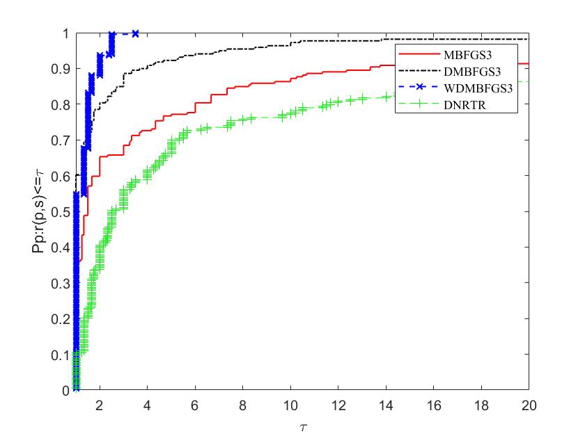
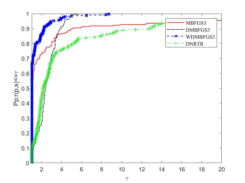
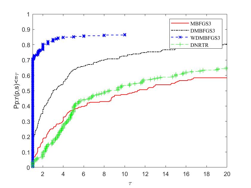
The figures illustrate the comparison on two aspects: the left side displays the percentage of the most efficient problems in the algorithm (), while the right side showcases the percentage of problems that the algorithm can solve ().For a given algorithm, the plot indicates its efficiency, while the plot represents its robustness.
To evaluate and compare the efficiency of these algorithms, we follow the methodology proposed by Dolan and More [17]. The parameters on the horizontal and vertical axes are defined as follows: "" represents the performance metric (NI, NFG, or CPU time), and the reciprocal of the ratio to the best performance among all methods is denoted as . The proportion of problems solved when the ratio of this method is less than parameter is indicated by . From Figures 7, 8 and 9, it can be seen that the performance of the DMBFGS3 algorithm is, in a sense, the best, because 59% of the problems are solved by this algorithm with the fewest number of iterations (NI), outperforming MBFGS3 and DNRTR, which solve at most 22% of the test problems. At the same time, Figure 7 shows that WDMBFGS3 solves 55% of the problems with the fewest number of iterations, although this result is not the optimal one. However, when we zoom in on the horizontal axis and expand the value to 3, WDMBFGS3 can solve nearly 100% of the problems, indicating that WDMBFGS3 has stronger robust stability. From the figure, it can be clearly seen that WDMBFGS3, using extrapolation techniques, consistently maintains the highest number of victories (indicating the highest probability of being the superior solver). Figure 8 shows that WDMBFGS3 solves 68% of the evaluation tasks with the fewest number of total function and gradient evaluations (NFG). Notably, when the horizontal axis is zoomed in to , DMBFGS3 and WDMBFGS3 perform excellently, solving over 90% of the problems. Although DMBFGS3’s performance in processing data is close to WDMBFGS3’s when , WDMBFGS3 solves these problems with fewer iterations (NI), so the algorithm with the extrapolation technique, WDMBFGS3, has a stronger advantage and competitiveness. Figure 9 shows the CPU time used by the algorithms, and it is clear that the WDMBFGS3 and DMBFGS3 algorithms significantly outperform the other two algorithms.
| DNRTR | MBFGS3 | DMBFGS3 | WDMBFGS3 | |||||
|---|---|---|---|---|---|---|---|---|
| #iter | cpu | #iter | cpu | #iter | cpu | #iter | cpu | |
| 900 | 34 | 0.046875 | 35 | 0.65625 | 41 | 0.03125 | 33 | 0.0625 |
| 1500 | 27 | 0.34375 | 35 | 2.078125 | 35 | 0.046875 | 42 | 0.0625 |
| 2100 | 28 | 2.25 | 35 | 12.54688 | 113 | 1.234375 | 51 | 0.09375 |
| Total | 89 | 2.640625 | 105 | 15.28125 | 189 | 1.3125 | 126 | 0.21875 |
Table 1 presents the outcomes from the issues with the quantity of variables within the interval (900, 2100). Observably, for extensive-scale unconstrained optimization challenges, the performance of the WDMBFGS3 algorithm is notably best than other algorithms.
4.3 Muskingum Model
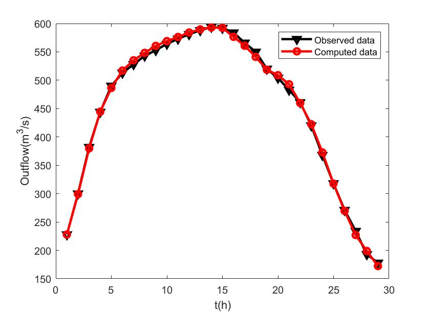
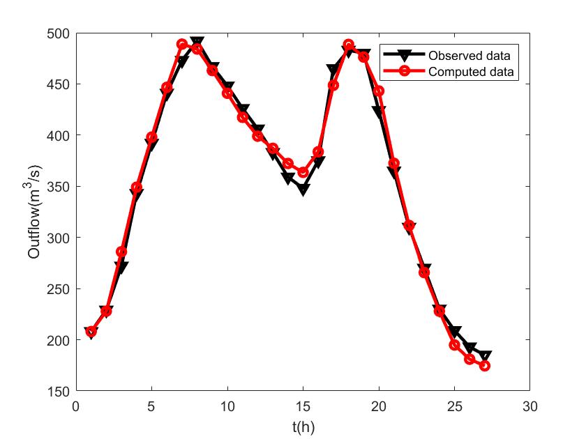
The nonlinear Muskingum model, frequently applied in hydrological engineering, addresses the challenges posed by optimization algorithms. A notable study by Ouyang et al.[31] presents this model, which is formulated as follows:
where: denotes the total time steps, is the storage time constant, is the weighting factor, is an additional parameter, represents the time step at time (), and are the observed inflow and outflow discharges, respectively.
We cited [32] as the source of the research data for this paper. The time step was set to 12 hours, and the initial parameter values were . Comprehensive information on and for 1961 is available in the work by Ouyang et al.[31]. Figure 11 displays both the recorded and computed outflows for the Muskingum model using the WDMBFGS3 in 1961, while Figure 11 presents the same for the DMBFGS3 in 1960. It is evident that the outflow curve fitted by the WDMBFGS algorithm is noticeably superior to that of the DMBFGS3.
5 Conclusion
This paper introduces an improved quasi-Newton algorithm, DMBFGS3, which incorporates diagonal transformations and an adjustment term on , further enhancing the stability of the algorithm. By introducing an extrapolation technique, the iterative process of the algorithm is accelerated, resulting in the proposed WDMBFGS3 algorithm. We discuss the performance of these two proposed algorithms in three different non-convex optimization experimental settings. A series of numerical experiments demonstrate that DMBFGS3 exhibits high efficiency and robustness when applied to non-convex optimization problems. Future research will focus on the following aspects: 1. Designing adaptive step sizes to avoid manual adjustments while ensuring theoretical convergence; 2. Investigating faster iterative setting strategies to improve the efficiency of model training.
Declarations
Data availability Data available on request from the authors.
Acknowledgement
This work is supported by Guangxi Science and Technology base and Talent Project (Grant No. AD22080047) and the special foundation for Guangxi Ba Gui Scholars.
References
- \bibcommenthead
- Wei et al. [2004] Wei, Z., Yu, G., Yuan, G., Lian, Z.: The superlinear convergence of a modified bfgs-type method for unconstrained optimization. Computational optimization and applications 29, 315–332 (2004)
- Davidon [1991] Davidon, W.C.: Variable metric method for minimization. SIAM Journal on optimization 1(1), 1–17 (1991)
- Li and Fukushima [2001] Li, D.-H., Fukushima, M.: A modified bfgs method and its global convergence in nonconvex minimization. Journal of Computational and Applied Mathematics 129(1-2), 15–35 (2001)
- Li and Fukushima [1999] Li, D., Fukushima, M.: A globally and superlinearly convergent gauss–newton-based bfgs method for symmetric nonlinear equations. SIAM Journal on numerical Analysis 37(1), 152–172 (1999)
- Li and Fukushima [2001] Li, D.-H., Fukushima, M.: On the global convergence of the bfgs method for nonconvex unconstrained optimization problems. SIAM Journal on Optimization 11(4), 1054–1064 (2001)
- Dennis and Moré [1974] Dennis, J.E., Moré, J.J.: A characterization of superlinear convergence and its application to quasi-newton methods. Mathematics of computation 28(126), 549–560 (1974)
- Griewank and Toint [1982] Griewank, A., Toint, P.L.: Local convergence analysis for partitioned quasi-newton updates. Numerische Mathematik 39(3), 429–448 (1982)
- Pierre [1986] Pierre, D.A.: Optimization Theory with Applications. Courier Corporation, ??? (1986)
- Andrei [2019] Andrei, N.: A diagonal quasi-newton updating method for unconstrained optimization. Numerical Algorithms 81(2), 575–590 (2019)
- Dennis and Wolkowicz [1993] Dennis, J.E. Jr, Wolkowicz, H.: Sizing and least-change secant methods. SIAM Journal on Numerical Analysis 30(5), 1291–1314 (1993)
- Wolfe [1969a] Wolfe, P.: Convergence conditions for ascent methods. SIAM review 11(2), 226–235 (1969)
- Wolfe [1969b] Wolfe, P.: Convergence conditions for ascent methods. SIAM review 11(2), 226–235 (1969)
- Chen et al. [2013] Chen, P., Huang, J., Zhang, X.: A primal–dual fixed point algorithm for convex separable minimization with applications to image restoration. Inverse Problems 29(2), 025011 (2013)
- Iiduka [2012] Iiduka, H.: Iterative algorithm for triple-hierarchical constrained nonconvex optimization problem and its application to network bandwidth allocation. SIAM Journal on Optimization 22(3), 862–878 (2012)
- Jolaoso et al. [2021] Jolaoso, L., Alakoya, T., Taiwo, A., Mewomo, O.: Inertial extragradient method via viscosity approximation approach for solving equilibrium problem in hilbert space. Optimization 70(2), 387–412 (2021)
- Abubakar et al. [2020a] Abubakar, J., Kumam, P., Hassan Ibrahim, A., Padcharoen, A.: Relaxed inertial tseng’s type method for solving the inclusion problem with application to image restoration. Mathematics 8(5), 818 (2020)
- Abubakar et al. [2020b] Abubakar, J., Kumam, P., Hassan Ibrahim, A., Padcharoen, A.: Relaxed inertial tseng’s type method for solving the inclusion problem with application to image restoration. Mathematics 8(5), 818 (2020)
- Abubakar et al. [2019] Abubakar, J., Sombut, K., Ibrahim, A.H., et al.: An accelerated subgradient extragradient algorithm for strongly pseudomonotone variational inequality problems. Thai Journal of Mathematics 18(1), 166–187 (2019)
- Alvarez [2004] Alvarez, F.: Weak convergence of a relaxed and inertial hybrid projection-proximal point algorithm for maximal monotone operators in hilbert space. SIAM Journal on Optimization 14(3), 773–782 (2004)
- Alvarez and Attouch [2001] Alvarez, F., Attouch, H.: An inertial proximal method for maximal monotone operators via discretization of a nonlinear oscillator with damping. Set-Valued Analysis 9, 3–11 (2001)
- Polyak [1964] Polyak, B.T.: Some methods of speeding up the convergence of iteration methods. Ussr computational mathematics and mathematical physics 4(5), 1–17 (1964)
- Alvarez [2000] Alvarez, F.: On the minimizing property of a second order dissipative system in hilbert spaces. SIAM Journal on Control and Optimization 38(4), 1102–1119 (2000)
- Sun and Liu [2015] Sun, M., Liu, J.: A modified hestenes–stiefel projection method for constrained nonlinear equations and its linear convergence rate. Journal of Applied Mathematics and Computing 49, 145–156 (2015)
- Ibrahim et al. [2022] Ibrahim, A.H., Kumam, P., Sun, M., Chaipunya, P., Abubakar, A.B.: Projection method with inertial step for nonlinear equations: application to signal recovery. Journal of Industrial and Management Optimization 19(1), 30–55 (2022)
- Moudafi and Elizabeth [2003] Moudafi, A., Elizabeth, E.: Approximate inertial proximal methods using the enlargement of maximal monotone operators. International Journal of Pure and Applied Mathematics 5(3), 283–299 (2003)
- Moudafi and Oliny [2003] Moudafi, A., Oliny, M.: Convergence of a splitting inertial proximal method for monotone operators. Journal of Computational and Applied Mathematics 155(2), 447–454 (2003)
- Andrei [2008] Andrei, N.: An unconstrained optimization test functions collection. Adv. Model. Optim 10(1), 147–161 (2008)
- Candès et al. [2006] Candès, E.J., Romberg, J., Tao, T.: Robust uncertainty principles: Exact signal reconstruction from highly incomplete frequency information. IEEE Transactions on information theory 52(2), 489–509 (2006)
- Donoho [2006] Donoho, D.L.: Compressed sensing. IEEE Transactions on information theory 52(4), 1289–1306 (2006)
- Aminifard et al. [2022] Aminifard, Z., Hosseini, A., Babaie-Kafaki, S.: Modified conjugate gradient method for solving sparse recovery problem with nonconvex penalty. Signal Processing 193, 108424 (2022)
- Ouyang et al. [2015] Ouyang, A., Liu, L.-B., Sheng, Z., Wu, F.: A class of parameter estimation methods for nonlinear muskingum model using hybrid invasive weed optimization algorithm. Mathematical Problems in Engineering 2015(1), 573894 (2015)
- Luo et al. [2022] Luo, D., Li, Y., Lu, J., Yuan, G.: A conjugate gradient algorithm based on double parameter scaled broyden–fletcher–goldfarb–shanno update for optimization problems and image restoration. Neural Computing and Applications 34(1), 535–553 (2022)