A definition of the asymptotic phase for quantum nonlinear oscillators from the Koopman operator viewpoint
Abstract
We propose a definition of the asymptotic phase for quantum nonlinear oscillators from the viewpoint of the Koopman operator theory. The asymptotic phase is a fundamental quantity for the analysis of classical limit-cycle oscillators, but it has not been defined explicitly for quantum nonlinear oscillators. In this study, we define the asymptotic phase for quantum oscillatory systems by using the eigenoperator of the backward Liouville operator associated with the fundamental oscillation frequency. By using the quantum van der Pol oscillator with Kerr effect as an example, we illustrate that the proposed asymptotic phase appropriately yields isochronous phase values in both semiclassical and strong quantum regimes.
Spontaneous rhythmic oscillations and synchronization are observed in a wide variety of classical rhythmic systems, and recent progress in nanotechnology is facilitating the analysis of quantum rhythmic systems. The asymptotic phase plays a fundamental role in the analysis of classical limit-cycle oscillators, but a fully quantum-mechanical definition for quantum limit-cycle oscillators has been lacking. In this study, we propose a definition of the asymptotic phase for quantum nonlinear oscillators, which naturally extends the definition of the asymptotic phase for classical stochastic oscillatory systems thomas2014asymptotic from the Koopman-operator viewpoint kato2021asymptotic and provides us with appropriate phase values for characterizing quantum synchronization.
I Introduction
Synchronization of spontaneous rhythmic oscillations are widely observed in nature winfree2001geometry ; kuramoto1984chemical ; pikovsky2001synchronization ; nakao2016phase ; ermentrout2010mathematical ; strogatz1994nonlinear . It has been extensively studied in a variety of classical systems in physics, chemistry, and biology. Recently, much progress has been made in the experimental realization of synchronization in micro- and nanoscale systems, such as nanoelectromechanical oscillators matheny2019exotic , micro lasers kreinberg2019mutual , spin torque oscillators singh2019mutual , and optomechanical oscillators colombano2019synchronization . Stimulated by the experimental developments, quantum synchronization has attracted much attention recently lee2013quantum ; walter2014quantum ; sonar2018squeezing ; kato2019semiclassical ; mok2020synchronization ; lee2014entanglement ; witthaut2017classical ; roulet2018quantum ; lorch2016genuine ; lorch2017quantum ; nigg2018observing ; weiss2016noise ; es2020synchronization ; kato2021enhancement ; kato2021instantaneous ; li2021quantum ; laskar2020observation ; koppenhofer2020quantum ; kato2020semiclassical ; hush2015spin ; weiss2017quantum ; mari2013measures ; xu2014synchronization ; roulet2018synchronizing ; chia2020relaxation ; arosh2021quantum ; jaseem2020generalized ; jaseem2020quantum ; cabot2021metastable and theoretical investigations of quantum signatures in synchronization, such as quantum fluctuations lee2013quantum ; walter2014quantum ; sonar2018squeezing ; kato2019semiclassical ; kato2020semiclassical , quantum entanglement lee2014entanglement ; witthaut2017classical ; roulet2018quantum , discrete nature of the energy spectrum lorch2016genuine ; lorch2017quantum ; nigg2018observing , and effects of quantum measurement weiss2016noise ; es2020synchronization ; kato2021enhancement ; kato2021instantaneous ; li2021quantum , have been carried out. Experimental realizations of quantum phase synchronization in spin- atoms laskar2020observation and on the IBM Q system koppenhofer2020quantum have also been reported recently.
In classical deterministic systems, spontaneous rhythmic oscillations are typically modeled as stable limit cycles of nonlinear dynamical systems. The asymptotic phase winfree2001geometry ; kuramoto1984chemical ; pikovsky2001synchronization ; nakao2016phase ; ermentrout2010mathematical , defined by the oscillator’s vector field and increases with a constant frequency in the basin of the limit cycle, plays a central role in analyzing synchronization properties of limit-cycle oscillators. It is the basis for phase reduction winfree2001geometry ; kuramoto1984chemical ; pikovsky2001synchronization ; nakao2016phase ; ermentrout2010mathematical ; strogatz1994nonlinear , which gives low-dimensional phase equations approximately describing the oscillators under weak perturbations. Recently, it has been clarified that the asymptotic phase, which was originally introduced from a geometrical viewpoint winfree2001geometry , has a natural relationship with the Koopman eigenfunction associated with the fundamental frequency of the oscillator mauroy2013isostables ; mauroy2020koopman ; shirasaka2017phase ; kuramoto2019concept ; kato2021asymptotic .
For classical stochastic oscillatory systems, Thomas and Lindner thomas2014asymptotic proposed a definition of the asymptotic phase in terms of the slowest decaying eigenfunction of the backward Fokker-Planck (Kolmogorov) operator describing the mean first passage time, which appropriately yields isochronous phase values that increase with a constant frequency on average even for strongly stochastic oscillations, in a similar way to the ordinary asymptotic phase for deterministic oscillators. We recently pointed out that their definition can be considered a natural extension of the deterministic definition from the Koopman operator viewpoint kato2021asymptotic (see junge2004uncertainty ; vcrnjaric2020koopman ; wanner2020robust for the details of the stochastic Koopman operator).
The classical definitions of the asymptotic phase are applicable to quantum nonlinear oscillators in the semiclassical regime, where the system is described by a stochastic differential equation for the phase-space state along a deterministic classical trajectory under the effect of small quantum noise kato2019semiclassical ; kato2020semiclassical ; kato2021asymptotic . However, in the stronger quantum regime, we cannot rely on the semiclassical approximation and how to define the asymptotic phase in a fully quantum-mechanical manner is an open question. In this study, we propose a definition of the asymptotic phase for quantum nonlinear oscillatory systems by using the eigenoperator of the adjoint Liouville operator, which is a counterpart of the backward Fokker-Planck operator in classical stochastic systems. We illustrate the validity of our definition by using a quantum van der Pol oscillator with quantum Kerr effect in both semiclassical and strong quantum regimes.
II Asymptotic phase for classical oscillatory systems
In this section, we briefly review the definitions of the asymptotic phase for deterministic winfree2001geometry ; kuramoto1984chemical ; pikovsky2001synchronization ; nakao2016phase ; ermentrout2010mathematical ; mauroy2020koopman ; shirasaka2017phase ; kuramoto2019concept and stochastic thomas2014asymptotic ; kato2021asymptotic classical oscillatory systems.
II.1 Deterministic oscillatory systems
Consider a deterministic dynamical system
| (1) |
where is the system state at time , is a vector field representing the system dynamics, and represents time derivative. We assume that this system has an exponentially stable limit-cycle solution with a natural period and frequency , satisfying , and denote its basin of attraction as . The asymptotic phase is defined such that is satisfied for , where represents the gradient with respect to winfree2001geometry ; kuramoto1984chemical ; pikovsky2001synchronization ; nakao2016phase ; ermentrout2010mathematical . The asymptotic phase of the system state then obeys
| (2) |
i.e., always increases with a constant frequency as evolves in . Thus, the asymptotic phase gives a nonlinear transformation of the system state to a phase value such that the dynamics of takes a simple linear form, The simplicity of the phase equation (2) has facilitated detailed studies of synchronization and collective dynamics in coupled-oscillator systems winfree2001geometry ; kuramoto1984chemical ; pikovsky2001synchronization ; nakao2016phase ; ermentrout2010mathematical . The level sets of are called isochrons.
The linear operator in the definition of the asymptotic phase is the infinitesimal generator of the Koopman operator describing the evolution of observables for the system described by Eq. (1) (see Refs. mauroy2013isostables ; mauroy2020koopman ; shirasaka2017phase ; kuramoto2019concept for details). The complex exponential of is an eigenfunction of with the eigenvalue , namely, it satisfies the eigenvalue equation . Therefore, the asymptotic phase has a natural operator-theoretic interpretation as the argument of the Koopman eigenfunction associated with the eigenvalue , characterized by the fundamental frequency of the oscillator mauroy2013isostables ; mauroy2020koopman ; shirasaka2017phase ; kuramoto2019concept . We can thus define the asymptotic phase by using the Koopman eigenfunction of as
| (3) |
II.2 Stochastic oscillatory systems
For stochastic oscillatory systems, we cannot use the deterministic limit-cycle solution in defining the asymptotic phase unless the noise is sufficiently weak. Thomas and Lindner thomas2014asymptotic defined the asymptotic phase for classical stochastic oscillators without relying on the deterministic limit cycle by using the eigenfunction with the slowest decay rate of the backward Fokker-Planck operator.
Consider a stochastic oscillator described by an Ito stochastic differential equation (SDE)
| (4) |
where is the system state at time , is a drift vector representing the deterministic dynamics, is a matrix characterizing the effect of the noise, and is a -dimensional Wiener process. This system is assumed to be oscillatory in the sense explained below. The transition probability density () of Eq. (4) obeys the forward and backward Fokker-Planck equations gardiner2009stochastic ,
| (5) |
and
| (6) |
respectively, where the (forward) Fokker-Planck operator is given by
| (7) |
and the backward Fokker-Planck operator is given by (in terms of )
| (8) |
Here, is a matrix of diffusion coefficients ( indicates matrix transposition). The forward and backward operators and are mutually adjoint, i.e., , where the inner product is defined as for two functions (the overline indicates complex conjugate and the integration is taken over the whole range of ).
As explained in Appendix A, the backward Fokker-Planck operator in Eq. (8) is the infinitesimal generator of the Koopman operator for Eq. (4). We denote the probability density function of at time as , which also obeys the Fokker-Planck equation , and an observable of the system at time as , which maps the system state to a complex value. The evolution of the expectation of the observable at can be expressed as
| (9) | ||||
| (10) |
where remains constant and evolves in the second expression, while remains constant and evolves in the last expression.
The linear differential operators and have a biorthogonal eigensystem of the eigenvalue and eigenfunctions and satisfying
| (11) |
where and represents the Kronecker delta gardiner2009stochastic . We assume that, among the eigenvalues, one eigenvalue is zero, which is associated with the stationary state of the system satisfying , and all other eigenvalues have negative real parts. It is assumed that the eigenvalues with the largest non-negative real part (or the smallest absolute real part, i.e., the slowest decay rate) are given by a complex-conjugate pair. We denote these eigenvalues as
| (12) |
where is the decay rate and represents the fundamental oscillation frequency of the system. The oscillatory property of the system is embodied in this assumption. We also assume that this pair of principal eigenvalues are well separated from other branches of eigenvalues and this oscillatory mode is dominant in the system.
Thomas and Lindner thomas2014asymptotic proposed a definition of the stochastic asymptotic phase of the system described by Eq. (4) by using the argument of the complex conjugate of the eigenfunction of associated with as (in the notation used here)
| (13) |
This definition is natural from the Koopman operator viewpoint kato2021asymptotic , as is the infinitesimal generator of the Koopman operator for Eq. (4) that formally goes back to the linear operator , i.e., to the infinitesimal generator of the Koopman operator for the deterministic system Eq. (1) in the noiseless limit . The exponential average of satisfies kato2021asymptotic
| (14) |
where represents the average over the stochastic trajectories of Eq. (4) starting from an initial point . Thus, the asymptotic phase defined by Eq. (13) increases with a constant frequency on average with the stochastic evolution of the system and can be considered a natural generalization of the deterministic asymptotic phase in Eq. (3). It is noted that we may also choose the eigenvalue and eigenfunction to define the stochastic asymptotic phase, which reverses its direction of increase.
III Asymptotic phase for quantum oscillatory systems
Our aim in this study is to propose a quantum-mechanical definition of the asymptotic phase that does not rely on classical trajectories. In Ref. kato2019semiclassical , we developed a semiclassical phase reduction theory for quantum limit-cycle oscillators, but the definition of the asymptotic phase was based on the deterministic limit cycle in the classical limit and could not be applied in stronger quantum regimes. In Ref. kato2021asymptotic , we considered the asymptotic phase of quantum limit-cycle oscillators using the definition for the classical stochastic oscillators explained in Sec. II, but it was valid only in the semiclassical regime. Here, we consider a quantum master equation describing the evolution of the density operator of the system and define the asymptotic phase by using the eigenoperator of the adjoint Liouville operator. We use standard notations for open quantum systems without a detailed explanation; see e.g., Refs. carmichael2007statistical ; gardiner1991quantum ; breuer2002theory for details.
III.1 Quantum master equation
We consider quantum oscillatory systems with a single degree of freedom coupled to reservoirs. The system’s quantum state is represented by a Hermitian density operator () and the observable is described by an operator , where represents Hermitian conjugate. Introducing an inner product of two operators and , the expectation of the observable is expressed as
| (15) |
In the Schrödinger picture, the quantum state evolves with time while the observable remains constant. Assuming that the interactions of the system with the reservoirs are instantaneous and Markovian approximation can be employed, the evolution of the density operator at time obeys the quantum master equation carmichael2007statistical ; gardiner1991quantum ; breuer2002theory
| (16) |
where the Liouville operator (sometimes called a superoperator because it acts on an operator) is given by
| (17) |
Here, is a system Hamiltonian, is a coupling operator between the system and th reservoir , is the commutator, is the Lindblad form, and the reduced Planck’s constant is set as .
In the Heisenberg picture, the quantum state remains constant while the observable evolves with time as
| (18) |
where the time dependence of is explicitly shown. Here, is the adjoint operator of satisfying
| (19) |
and can be explicitly calculated as
| (20) |
where is the adjoint Lindblad form breuer2002theory . The evolution of the expectation of with respect to at can be expressed as
| (21) | ||||
| (22) |
where remains constant and evolves in the second expression (Schrödinger picture), while remains constant and evolves in the last expression (Heisenberg picture). Equation (22) corresponds to Eq. (10) for the expectation of the observable for classical stochastic systems. Thus, the adjoint operator is a counterpart of the backward Fokker-Planck operator in Sec. II, namely, corresponds to the infinitesimal generator of the Koopman operator.
We assume that the operators and have a biorthogonal eigensystem consisting of the eigenvalue and right and left eigenoperators and , satisfying
| (23) |
for li2014perturbative . Among the eigenvalues, one eigenvalue is always , which is associated with the stationary state of the system satisfying , and all other eigenvalues have negative real parts; This also indicates that the system has no decoherece free subspace lidar1998decoherence . We assume that, reflecting the system’s oscillatory dynamics, the eigenvalues with the largest non-vanishing real part (i.e., with the slowest decay rate) are given by a complex-conjugate pair. We denote these eigenvalues as
| (24) |
where is the decay rate and gives the fundamental frequency of the oscillation. As in the case of the stochastic oscillatory systems in Sec. II, the oscillatory property of the system is embodied in this assumption.
III.2 Phase space representation
The density operator can also be represented by using quasiprobability distributions in the phase space such as the , , and Wigner distributions carmichael2007statistical ; gardiner1991quantum ; cahill1969density . We use the representation and express as
| (25) |
where is a coherent state specified by a complex value , or equivalently by a complex vector , is a quasiprobability distribution of , , and the integral is taken over . Defining the representation of an observable as
| (26) |
where is expressed in the normal order carmichael2007statistical ; gardiner1991quantum ; cahill1969density , the expectation of is expressed as
| (27) |
Here, we defined the inner product of two functions , , where the integral is taken over the complex plane.
In the Schrödinger picture, the time evolution of (dependence on is explicitly denoted) corresponding to the master equation (16) is describied by a partial differential equation
| (28) |
where the differential operator is related to the Liouville operator in Eq. (16) via
and can be explicitly calculated from Eq. (16) by using the standard calculus for the phase-space representation carmichael2007statistical ; gardiner1991quantum ; cahill1969density .
The corresponding evolution of the representation of the observable in the Heisenberg picture is given by
| (29) |
where the differential operator is the adjoint of , i.e.,
| (30) |
and satisfies
| (31) |
Thus, is the generator of the Koopman operator in the representation describing the evolution of , which corresponds to the adjoint Liouville operator in Eq. (20).
Corresponding to the Liouville operators and , the differential operators and also possess a biorthogonal eigensystem of eigenvalue and eigenfunctions and , satisfying
| (32) |
which has one-to-one correspondence with Eq. (23). The eigenvalues are the same as those of , and the eigenfunctions and of are related to the eigenoperators and of via
| (33) |
which follow from
| (34) |
and
| (35) |
III.3 Quantum asymptotic phase
Generalizing the definition for classical stochastic oscillatory systems in Sec. II, we here propose a definition of the quantum asymptotic phase. We note that, in quantum systems, the system state is given by the density operator and individual trajectories as in the classical stochastic systems cannot be considered.
First, we define the quantum asymptotic phase of the coherent state in the representation. Considering the definition Eq. (13) of the asymptotic phase in terms of the eigenfunction of the backward Fokker-Planck operator in the classical stochastic case, we define the quantum asymptotic phase as the argument of the complex conjugate of the eigenfunction in the representation associated with the principal eigenvalue as
| (36) |
Next, considering that the general quantum state is represented as a superposition of coherent states with the weight , Eq. (25), we define the asymptotic phase of as
| (37) |
It can be shown that the asymptotic phase evolves with a constant frequency as the quantum state evolves according to the master equation (16). Defining
| (38) |
where the dependence on time is explicitly denoted, we have
| (39) | ||||
| (40) |
or, equivalently,
| (41) | ||||
| (42) |
Integrating by time, we obtain
| (43) |
where is the initial state at , and hence the asymptotic phase is given by
| (44) |
Differentiating by , we obtain
| (45) |
namely, the asymptotic phase increases with a constant frequency with the evolution of the quantum state .
Thus, by using the eigenfunction of the adjoint linear operator or equivalently the eigenoperator of the adjoint operator associated with the eigenvalue , we can define the asymptotic phase of the quantum state . The quantum master equation (16), adjoint Liouville operator (or adjoint differential operator in the representation), and eigenoperator (or the eigenfunction in the representation) with the eigenvalue correspond to the forward Fokker-Planck equation (5), backward Fokker-Planck operator , and eigenfunction with the eigenvalue in the classical stochastic system discussed in Sec. II, respectively.
We stress, however, that the system state is generally represented by the density operator or quasiprobability distribution and individual trajectories cannot be considered in the quantum case. As in the classical stochastic case, we may also choose the eigenvalue , eigenfunction , and eigenoperator to define the quantum asymptotic phase, which reverses its direction of increase.
IV Example: quantum van der Pol oscillator
In this section, using the quantum van der Pol model with quantum Kerr effect as an example, we illustrate the validity of the quantum asymptotic phase defined in Sec. III. We also analyze a damped harmonic oscillator in Appendix D.
IV.1 Quantum van der Pol model with quantum Kerr effect
As an example of quantum oscillatory systems, we consider the quantum van der Pol model with quantum Kerr effect. The system’s density operator obeys the master equation
| (46) |
where and are annihilation and creation operators, is the Hamiltonian, is the frequency parameter of the oscillator, is the Kerr parameter, and and are the decay rates for negative damping and nonlinear damping, respectively kato2020semiclassical ; lorch2016genuine . By using the standard rule of calculus carmichael2007statistical ; gardiner1991quantum ; cahill1969density , we can derive the differential operator in Eq. (28) describing the evolution of the representation of from the Liouville operator , which consists of third- and higher-order derivative with respect to lorch2016genuine .
To evaluate the fundamental frequency and the asymptotic phase of the system, we numerically calculate the eigenvalues and eigenfunctions of the Liouville and adjoint Liouville operators and . To this end, we approximately truncate the number representation of the density operator as a large matrix and map it to a -dimensional vector of the double-ket notation albert2018lindbladians . We can then approximately represent the Liouville operators and by matrices and calculate their eigensystem to obtain the asymptotic phase in Eq. (36).
IV.2 Semiclassical regime
We first consider the semiclassical regime where and are sufficiently small. In this case, as explained in Appendix B, we can approximate Eq. (28) by a Fokker-Planck equation for , namely, the system state is approximately equivalent to a classical stochastic system. Furthermore, in the classical limit where the quantum noise vanishes, the system is described by a single complex variable obeying a deterministic ordinary differential equation
| (47) |
This equation represents the Stuart-Landau oscillator (normal form of the supercritical Hopf bifurcation) kuramoto1984chemical and possesses a stable limit-cycle solution , which is represented as a function of the phase with a natural frequency and radius . The basin of this limit cycle is the whole complex plane except the origin. The classical asymptotic phase of this system is given by kato2019semiclassical
| (48) |
and satisfies as evolves in under Eq. (47) nakao2016phase . As stated in Sec. II, this is the argument of the Koopman eigenfunction of the system associated with the eigenvalue . In Ref. kato2019semiclassical , we used this for the phase-reduction analysis of quantum synchronization in the semiclassical regime with weak quantum noise. It is expected that the quantum asymptotic phase of the coherent state is close to the classical asymptotic phase when the quantum noise is sufficiently small.
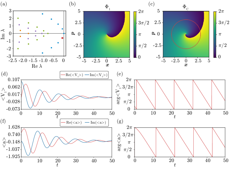
Figure 1(a) shows the eigenvalues of near the imaginary axis obtained numerically, where the principal eigenvalue is shown by a red dot (), and Figs. 1(b) and 1(c) compare the quantum-mechanical phase with the corresponding classical phase . Here, we adopt a negative value for so that the resulting phase increases in the counterclockwise direction from to on the complex plane, i.e., satisfies where and is a circle around .
As the quantum noise is small, the quantum frequency and the asymptotic phase obtained numerically from are close to the classical frequency and asymptotic phase , respectively. The difference between and arises from the small quantum noise; in the limit of vanishing quantum noise, the eigenfunction of in the representation coincides with the Koopman eigenfunction of the deterministic system Eq. (47) with the eigenvalue and therefore reproduces the classical phase (see Appendix C). Here, we note that the principal eigenvalues and are well separated from other branches of eigenvalues with faster decay rates and the corresponding oscillatory modes become quickly dominant.
To demonstrate that the present definition of the quantum asymptotic phase yields appropriate values, we consider free oscillatory relaxation of from a coherent initial state with at and measure . For comparison, we also measure the argument of the expectation of the annihilation operator , which simply gives the polar angle of on the complex plane. We note that, although the system state starts from a pure coherent state, it soon becomes a mixed state due to the coupling with the reservoirs and eventually relaxes to the stationary state .
Figures 1(d) and (e) plot the evolution of the expectation of the eigenoperator and the quantum asymptotic phase , respectively, and Figs. 1(f) and (g) show the evolution of the expectation and its polar angle , respectively. The asymptotic phase increases with a constant frequency and appropriately yields isochronous phase values. In contrast, the polar angle does not increase constantly with time, in particular in the transient process before , as shown in Fig. 1(g); as the limit cycle in the classical limit is rotationally symmetric in this model, the polar angle also yields almost constantly increasing phase values after relaxation.
Thus, the quantum asymptotic phase increases with a constant frequency in the semiclassical regime of a quantum van der Pol model with the quantum Kerr effect.
IV.3 Strong quantum regime
Next, we consider a strong quantum regime with relatively large and , where only a small number of energy states participates in the system dynamics and the semiclassical description is not valid. The eigenvalues of obtained numerically are shown in Fig. 2(a). Figures 2(b) and 2(c) show the quantum-mechanical phase and the corresponding classical phase . Because the system is in the strong quantum regime, is distinctly different from and the classical frequency also differs largely from the true quantum frequency . Here, we again note that the principal eigenvalues have much smaller (less than half of the second largest) decay rate than the eigenvalues in the other branches.
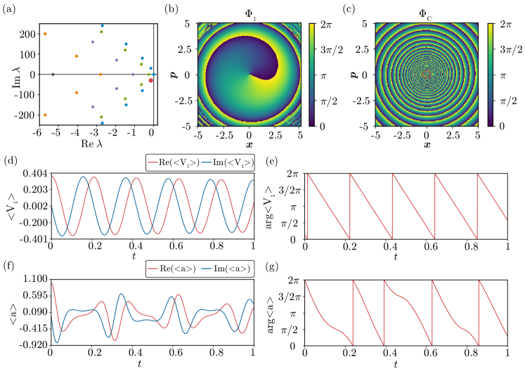
We consider free oscillatory relaxation of from a coherent initial state with at and measure the evolution of the asymptotic phase of the system state . For comparison, we also measure the polar angle of .
Figures 2(d) and (e) plot the evolution of the expectation of the eigenoperator and the quantum asymptotic phase , respectively, and Figs. 2(f) and (g) show the evolution of the expectation and its polar angle , respectively. As expected, the asymptotic phase appropriately gives constantly varying phase values with the frequency . In contrast, the polar angle does not vary constantly with time and is not isochronous. This is because the transition between relatively a small number of energy levels takes part in the system dynamics and the discreteness of the energy spectra can play important roles in this strong quantum regime.
Thus, the quantum asymptotic phase gives appropriate phase values that increase with a constant frequency even in the strong quantum regime of a quantum van der Pol model with quantum Kerr effect, even though the strong quantum effect strongly alters the dynamics of the system from the classical limit.
IV.4 Fundamental difference between the classical and quantum systems
Although we introduced the definition of the quantum asymptotic phase by analogy with the classical deterministic phase and classical stochastic asymptotic phase , a fundamental difference exists between the quantum and classical cases. Specifically, in the quantum case, the system state is described by the density operator and the asymptotic phase assigns a phase value on each , while in the classical case, the phase function or assigns a phase value on each individual state , although the probability density function is used in defining the stochastic asymptotic phase . This difference arises because the system state can be described by a SDE representing a single stochastic trajectory of the noisy oscillator in the classical stochastic case, whereas the system state can only be characterized by the density operator representing the statistical state of the system in the quantum case.
Though we have taken the viewpoint that the asymptotic phase is defined for a single stochastic trajectory in the classical stochastic case in this study, we may also consider that the asymptotic phase is defined for the probability density rather than for the state in the classical stochastic case. Then, the quantum asymptotic phase as a function of the density matrix corresponds to the stochastic asymptotic phase as a function of the probability density in the classical stochastic case in Sec. II. We regarded this quantity as the exponential average of the asymptotic phase values defined for individual states in Eq. (14).
In the present approach, it is always possible to formally introduce a ’phase function’ for any oscillatory system as long as it has the decaying mode with a non-zero imaginary part by using the associated eigenoperator. However, this phase function does not necessarily play the role of a quantum asymptotic phase unless the system exhibits limit-cycle oscillations and synchronization. As an example, in Appendix D, we introduce a phase function of a damped quantum harmonic oscillator, which cannot be considered the quantum asymptotic phase since the system does not exhibit synchronization. Only when the system is nonlinear and exhibits synchronization, the asymptotic phase captures the synchronization dynamics of the system.
The asymptotic phase is the basis for developing phase reduction theory for classical nonlinear oscillators. For quantum oscillatory systems, however, even if we can introduce the asymptotic phase as described in this study, it does not necessarily mean that we can develop the phase reduction theory. This is because the quantum state may not be appropriately localized in the phase-space representation and hence it may not be reconstructed from the phase value even approximately. Still, as we showed for the case of the quantum vdP oscillator in the semiclassical regime kato2019semiclassical , we may approximately describe the dynamics of the quantum state by using the reduced phase equation and perform a detailed synchronization analysis in appropriate physical situations. It should be noted that we also encounter a similar problem in developing phase reduction theory for classical oscillators under strong noise. We also note that, even if we cannot derive a reduced phase description for quantum nonlinear oscillators, the asymptotic phase can be used to characterize the peculiar properties of quantum synchronization kato2021koopman2 .
V Summary
In this study, we proposed a definition of the asymptotic phase for quantum oscillatory systems by generalizing the asymptotic phase for classical stochastic oscillatory system proposed by Thomas and Lindner thomas2014asymptotic from the Koopman operator viewpoint kato2021asymptotic . The proposed asymptotic phase is defined by using the eigenoperator of the adjoint Liouville operator describing the evolution of the quantum-mechanical observable, in close analogy to the asymptotic phase for classical limit-cycle oscillators that can be interpreted as the argument of the Koopman eigenfunction associated with the fundamental frequency. By using the quantum van der Pol model with quantum Kerr effect as an example, we demonstrated that the proposed asymptotic phase appropriately yields isochronous phase values even in the strong quantum regime where the semiclassical approximation is not valid.
Though quantum synchronization has attracted much attention recently, compared with classical synchronization, systematic analysis of the quantum synchronization has been restricted, partly due to the lack of the clear definition of the phase. The proposed definition of the asymptotic phase valid in strong quantum regimes may be used for systematic and quantitative analysis of synchronization phenomena in quantum nonlinear oscillators kato2021koopman2 . Moreover, we may be able to develop a phase reduction theory for strongly quantum nonlinear oscillators by using the proposed definition, which would allow us to reduce the system dynamics to a simple phase equation and facilitates detailed analysis, control, and optimization of quantum nonlinear oscillators. It will also be interesting to extend the definition of the amplitude functions for classical stochastic oscillators perez2021isostables ; kato2021asymptotic to strongly quantum oscillatory systems on the basis of the Koopman operator theory.
Acknowledgements.
The authors thank anonymous reviewers for their enlightning comments. Numerical simulations have been performed by using QuTiP numerical toolbox johansson2012qutip ; johansson2013qutip . This research was funded by JSPS KAKENHI JP17H03279, JP18H03287, JPJSBP120202201, JP20J13778, JP22K14274, JP22K11919, JP22H00516 and JST CREST JP-MJCR1913.Data availability
The data that supports the findings of this study are available within the article.
Appendix A Koopman operator for classical stochastic processes
In this section, we briefly summarize the definition of the Koopman operator for classical stochastic processes described by the Ito SDE (4). The evolution of an observable for this Ito diffusion process from time to is expressed as mezic2005spectral ; oksendal2013stochastic ; vcrnjaric2020koopman
| (49) |
where () is the stochastic Koopman operator defined as
| (50) | ||||
| (51) |
Here, represents the expectation over the stochastic realizations of started from at , () is the transition probability density, and represents the inner product defined in Sec. II. Defining a time evolution operator (), the evolution of the probability density is expressed as
| (52) |
where the operation of on a function is given by
| (53) |
The Koopman operator is the adjoint of , i.e.,
| (54) | ||||
| (55) | ||||
| (56) |
for two functions . It is noted that the expectation of the observable at time can be expressed as
| (57) | ||||
| (58) |
It can be shown that the infinitesimal generator of is given by the backward operator in Eq. (8) (see e.g. Ref. oksendal2013stochastic for a rigorous treatment). From the Ito formula gardiner2009stochastic ; oksendal2013stochastic , the SDE for a function is given by
| (59) |
which gives
| (60) |
by integration. Assuming the function to be the observable at , the infinitesimal evolution of at can be represented as
| (61) |
Thus, we can express the Koopman operator as .
From the adjoint relation for and , and are also adjoint to each other, i.e., , and the evolution of the expectation of the observable at time can be expressed as in Eq. (10).
Appendix B Quantum van der Pol oscillator with Kerr effect in the semiclassical regime
In this section, we briefly explain the classical limit of the quantum van der Pol oscillator. As shown in Ref. kato2019semiclassical , in the semiclassical regime, the linear operator in Eq. (28) describing the evolution of the quasiprobability distribution in the representation of the quantum van der Pol oscillator can be approximated by a Fokker-Planck operator
| (62) |
by neglecting the third- and higher-order derivatives, where and . The drift vector and the matrix are given by
| (63) | ||||
| (64) |
The corresponding stochastic differential equation is thus given by
| (65) |
where and are independent Wiener processes and the matrix is given by
| (66) |
where . It is noted that the two equations for and in Eq. (65) are mutually complex conjugate and represent the same dynamics.
In the classical limit, the deterministic part of Eq. (65) gives the Stuart-Landau equation for the complex variable given in Eq. (47), which is analytically solvable and the asymptotic phase can be explicitly obtained as given in Eq. (48) kuramoto1984chemical ; nakao2016phase .
Appendix C Classical limit of the quantum asymptotic phase
In this section, we explain that the quantum asymptotic phase formally reproduces the deterministic asymptotic phase in the classical limit. In the semiclassical regime, the linear operator of Eq. (28) for the quasiprobability distribution in the representation can be approximated by a Fokker-Planck operator of the form Eq. (62). By introducing a real vector and the corresponding probability density function , the Fokker-Planck operator for can be cast into a real Fokker-Planck operator for in Eq. (7).
In the classical limit, the quantum noise vanishes and the diffusion term in disappears. Thus, formally becomes a classical Liouville operator, i.e., , and the corresponding backward Liouville operator formally becomes the infinitesimal generator of the deterministic Koopman operator, i.e., . Also, the decay rate approaches and the eigenvalue approaches where is the frequency of the limiting classical deterministic system. As discussed in Sec. II A, the classical asymptotic phase is obtained as the argument of the eigenfunction of associated with the eigenvalue . Thus, the quantum asymptotic phase formally reproduces the deterministic asymptotic phase in the classical limit with vanishing quantum noise.
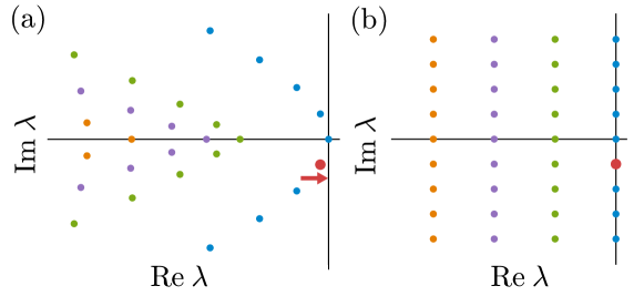
Figure 3 schematically shows the behavior of the eigenvalues of approaching those of the deterministic system in the classical limit with a stable limit-cycle solution. The eigenvalues in the classical limit are given in the form and , where is the real part of the largest non-zero eigenvalue and is the imaginary part of the pure-imaginary eigenvalue with the smallest absolute imaginary part. In the example of a quantum van der Pol oscillator with quantum Kerr effect in Sec. IV, and . As the system approaches the classical limit, each curved branch of eigenvalues of in Fig. 3(a) approaches the corresponding straight branch of eigenvalues in Fig. 3(b) in the classical limit.
The above formal correspondence with the conventional definition of the asymptotic phase in the classical limit supports the validity of our definition of the quantum asymptotic phase.
Appendix D Phase function of a quantum damped harmonic oscillator
In Ref. thomas2019phase , Thomas and Lindner considered the stochastic phase function for a classical damped harmonic oscillator described by a multi-dimensional Ornstein-Uhlenbeck process. In this section, generalizing their result, we consider a simple quantum harmonic oscillator with a damping and formally calculate the phase function. This system is linear and does not possess a limit cycle in the classical limit, but the isochronous phase function as defined in Sec. III can still be introduced (as the system lacks an asymptotic periodic orbit in this case, we do not use the term ’asymptotic’).
The eigenoperator of the adjoint Liouville operator can be analytically obtained in this case. The evolution of a damped harmonic oscillator is described by a quantum master equation
| (67) |
where is the natural frequency of the system, denotes the decay rate for the linear damping, and is the Lindblad form carmichael2007statistical . The eigenoperator associated with the slowest non-vanishing decay rate of the adjoint Liouville operator of is simply given by , i.e., , where barnett2000spectral ; briegel1993quantum . Therefore, the phase function of the coherent state is given by
| (68) |
where , and the phase function of the density operator at time is given by
| (69) |
For the initial condition with , the expectation of evolves as
| (70) |
which gives . Thus, the phase of the state is given by
| (71) |
which decreases with a constant frequency .
As shown in this example of a quantum damped harmonic oscillator, we can formally introduce the phase function for a wide class of oscillators, even if the system does not exhibit limit-cycle dynamics. In a special case where the system exhibits limit-cycle dynamics, our definition of the phase function plays the role of the quantum asymptotic phase.
References
- (1) Peter J Thomas and Benjamin Lindner. Asymptotic phase for stochastic oscillators. Physical Review Letters, 113(25):254101, 2014.
- (2) Yuzuru Kato, Jinjie Zhu, Wataru Kurebayashi, and Hiroya Nakao. Asymptotic phase and amplitude for classical and semiclassical stochastic oscillators via koopman operator theory. Mathematics, 9(18):2188, 2021.
- (3) Arthur T Winfree. The geometry of biological time. Springer, New York, 2001.
- (4) Yoshiki Kuramoto. Chemical oscillations, waves, and turbulence. Springer, Berlin, 1984.
- (5) Arkady Pikovsky, Michael Rosenblum, and Jürgen Kurths. Synchronization: a universal concept in nonlinear sciences. Cambridge University Press, Cambridge, 2001.
- (6) Hiroya Nakao. Phase reduction approach to synchronisation of nonlinear oscillators. Contemporary Physics, 57(2):188–214, 2016.
- (7) G Bard Ermentrout and David H Terman. Mathematical foundations of neuroscience. Springer, New York, 2010.
- (8) SH Strogatz. Nonlinear dynamics and chaos. Westview Press, 1994.
- (9) Matthew H Matheny, Jeffrey Emenheiser, Warren Fon, Airlie Chapman, Anastasiya Salova, Martin Rohden, Jarvis Li, Mathias Hudoba de Badyn, Márton Pósfai, Leonardo Duenas-Osorio, et al. Exotic states in a simple network of nanoelectromechanical oscillators. Science, 363(6431):eaav7932, 2019.
- (10) Sören Kreinberg, Xavier Porte, David Schicke, Benjamin Lingnau, Christian Schneider, Sven Höfling, Ido Kanter, Kathy Lüdge, and Stephan Reitzenstein. Mutual coupling and synchronization of optically coupled quantum-dot micropillar lasers at ultra-low light levels. Nature communications, 10(1):1539, 2019.
- (11) Hanuman Singh, S Bhuktare, A Bose, A Fukushima, K Yakushiji, S Yuasa, H Kubota, and Ashwin A Tulapurkar. Mutual synchronization of spin-torque nano-oscillators via oersted magnetic fields created by waveguides. Physical Review Applied, 11(5):054028, 2019.
- (12) MF Colombano, G Arregui, NE Capuj, A Pitanti, J Maire, A Griol, B Garrido, A Martinez, CM Sotomayor-Torres, and D Navarro-Urrios. Synchronization of optomechanical nanobeams by mechanical interaction. Physical Review Letters, 123(1):017402, 2019.
- (13) Tony E Lee and HR Sadeghpour. Quantum synchronization of quantum van der pol oscillators with trapped ions. Physical Review Letters, 111(23):234101, 2013.
- (14) Stefan Walter, Andreas Nunnenkamp, and Christoph Bruder. Quantum synchronization of a driven self-sustained oscillator. Physical Review Letters, 112(9):094102, 2014.
- (15) Sameer Sonar, Michal Hajdušek, Manas Mukherjee, Rosario Fazio, Vlatko Vedral, Sai Vinjanampathy, and Leong-Chuan Kwek. Squeezing enhances quantum synchronization. Physical Review Letters, 120(16):163601, 2018.
- (16) Yuzuru Kato, Naoki Yamamoto, and Hiroya Nakao. Semiclassical phase reduction theory for quantum synchronization. Phys. Rev. Research, 1:033012, Oct 2019.
- (17) W-K Mok, L-C Kwek, and H Heimonen. Synchronization boost with single-photon dissipation in the deep quantum regime. Physical Review Research, 2(3):033422, 2020.
- (18) Tony E Lee, Ching-Kit Chan, and Shenshen Wang. Entanglement tongue and quantum synchronization of disordered oscillators. Physical Review E, 89(2):022913, 2014.
- (19) Dirk Witthaut, Sandro Wimberger, Raffaella Burioni, and Marc Timme. Classical synchronization indicates persistent entanglement in isolated quantum systems. Nature Communications, 8:14829, 2017.
- (20) Alexandre Roulet and Christoph Bruder. Quantum synchronization and entanglement generation. Physical Review Letters, 121(6):063601, 2018.
- (21) Niels Lörch, Ehud Amitai, Andreas Nunnenkamp, and Christoph Bruder. Genuine quantum signatures in synchronization of anharmonic self-oscillators. Physical Review Letters, 117(7):073601, 2016.
- (22) Niels Lörch, Simon E Nigg, Andreas Nunnenkamp, Rakesh P Tiwari, and Christoph Bruder. Quantum synchronization blockade: Energy quantization hinders synchronization of identical oscillators. Physical Review Letters, 118(24):243602, 2017.
- (23) Simon E Nigg. Observing quantum synchronization blockade in circuit quantum electrodynamics. Physical Review A, 97(1):013811, 2018.
- (24) Talitha Weiss, Andreas Kronwald, and Florian Marquardt. Noise-induced transitions in optomechanical synchronization. New Journal of Physics, 18(1):013043, 2016.
- (25) Najmeh Es’ haqi Sani, Gonzalo Manzano, Roberta Zambrini, and Rosario Fazio. Synchronization along quantum trajectories. Physical Review Research, 2(2):023101, 2020.
- (26) Yuzuru Kato and Hiroya Nakao. Enhancement of quantum synchronization via continuous measurement and feedback control. New Journal of Physics, 23(1):013007, 2021.
- (27) Yuzuru Kato and Hiroya Nakao. Instantaneous phase synchronization of two decoupled quantum limit-cycle oscillators induced by conditional photon detection. Physical Review Research, 3(1):013085, 2021.
- (28) Wenlin Li, Najmeh Es’ haqi Sani, Wen-Zhao Zhang, and David Vitali. Quantum zeno effect in self-sustaining systems: Suppressing phase diffusion via repeated measurements. Physical Review A, 103(4):043715, 2021.
- (29) Arif Warsi Laskar, Pratik Adhikary, Suprodip Mondal, Parag Katiyar, Sai Vinjanampathy, and Saikat Ghosh. Observation of quantum phase synchronization in spin-1 atoms. Physical Review Letters, 125(1):013601, 2020.
- (30) Martin Koppenhöfer, Christoph Bruder, and Alexandre Roulet. Quantum synchronization on the ibm q system. Physical Review Research, 2(2):023026, 2020.
- (31) Yuzuru Kato and Hiroya Nakao. Semiclassical optimization of entrainment stability and phase coherence in weakly forced quantum limit-cycle oscillators. Physical Review E, 101(1):012210, 2020.
- (32) Michael R Hush, Weibin Li, Sam Genway, Igor Lesanovsky, and Andrew D Armour. Spin correlations as a probe of quantum synchronization in trapped-ion phonon lasers. Physical Review A, 91(6):061401, 2015.
- (33) Talitha Weiss, Stefan Walter, and Florian Marquardt. Quantum-coherent phase oscillations in synchronization. Physical Review A, 95(4):041802, 2017.
- (34) A Mari, A Farace, N Didier, V Giovannetti, and R Fazio. Measures of quantum synchronization in continuous variable systems. Physical Review Letters, 111(10):103605, 2013.
- (35) Minghui Xu, David A Tieri, EC Fine, James K Thompson, and Murray J Holland. Synchronization of two ensembles of atoms. Physical Review Letters, 113(15):154101, 2014.
- (36) Alexandre Roulet and Christoph Bruder. Synchronizing the smallest possible system. Physical Review Letters, 121(6):053601, 2018.
- (37) A Chia, LC Kwek, and C Noh. Relaxation oscillations and frequency entrainment in quantum mechanics. Physical Review E, 102(4):042213, 2020.
- (38) Lior Ben Arosh, MC Cross, and Ron Lifshitz. Quantum limit cycles and the rayleigh and van der pol oscillators. Physical Review Research, 3(1):013130, 2021.
- (39) Noufal Jaseem, Michal Hajdušek, Parvinder Solanki, Leong-Chuan Kwek, Rosario Fazio, and Sai Vinjanampathy. Generalized measure of quantum synchronization. Physical Review Research, 2(4):043287, 2020.
- (40) Noufal Jaseem, Michal Hajdušek, Vlatko Vedral, Rosario Fazio, Leong-Chuan Kwek, and Sai Vinjanampathy. Quantum synchronization in nanoscale heat engines. Physical Review E, 101(2):020201, 2020.
- (41) Albert Cabot, Gian Luca Giorgi, and Roberta Zambrini. Metastable quantum entrainment. New Journal of Physics, 23(10):103017, 2021.
- (42) Alexandre Mauroy, Igor Mezić, and Jeff Moehlis. Isostables, isochrons, and koopman spectrum for the action–angle representation of stable fixed point dynamics. Physica D: Nonlinear Phenomena, 261:19–30, 2013.
- (43) Y Susuki Mauroy and I Mezic. The koopman operator in systems and control, 2020.
- (44) Sho Shirasaka, Wataru Kurebayashi, and Hiroya Nakao. Phase-amplitude reduction of transient dynamics far from attractors for limit-cycling systems. Chaos, 27(2):023119, 2017.
- (45) Yoshiki Kuramoto and Hiroya Nakao. On the concept of dynamical reduction: the case of coupled oscillators. Philosophical Transactions of the Royal Society A, 377(2160):20190041, 2019.
- (46) Oliver Junge, Jerrold E Marsden, and Igor Mezic. Uncertainty in the dynamics of conservative maps. In 2004 43rd IEEE Conference on Decision and Control (CDC)(IEEE Cat. No. 04CH37601), volume 2, pages 2225–2230. IEEE, 2004.
- (47) Nelida Črnjarić-Žic, Senka Maćešić, and Igor Mezić. Koopman operator spectrum for random dynamical systems. Journal of Nonlinear Science, 30(5):2007–2056, 2020.
- (48) Mathias Thomas Wanner. Robust Approximation of the Stochastic Koopman Operator. University of California, Santa Barbara, 2020.
- (49) Crispin Gardiner. Stochastic methods, volume 4. Springer Berlin, 2009.
- (50) Daniel A Lidar, Isaac L Chuang, and K Birgitta Whaley. Decoherence-free subspaces for quantum computation. Physical Review Letters, 81(12):2594, 1998.
- (51) Howard J Carmichael. Statistical Methods in Quantum Optics 1, 2. Springer, New York, 2007.
- (52) Crispin W Gardiner. Quantum Noise. Springer, New York, 1991.
- (53) Heinz-Peter Breuer, Francesco Petruccione, et al. The theory of open quantum systems. Oxford University Press on Demand, 2002.
- (54) Andy CY Li, F Petruccione, and Jens Koch. Perturbative approach to markovian open quantum systems. Scientific reports, 4:4887, 2014.
- (55) Kevin E Cahill and Roy J Glauber. Density operators and quasiprobability distributions. Physical Review, 177(5):1882, 1969.
- (56) Victor V Albert. Lindbladians with multiple steady states: theory and applications. arXiv preprint arXiv:1802.00010, 2018.
- (57) Yuzuru Kato and Hiroya Nakao. Quantum asymptotic phase reveals signatures of quantum synchronization. New Journal of Physics, 25:023012, 2023.
- (58) Alberto Pérez-Cervera, Benjamin Lindner, and Peter J Thomas. Isostables for stochastic oscillators. Physical review letters, 127(25):254101, 2021.
- (59) JR Johansson, PD Nation, and Franco Nori. Qutip: An open-source python framework for the dynamics of open quantum systems. Computer Physics Communications, 183(8):1760–1772, 2012.
- (60) JR Johansson, PD Nation, and Franco Nori. Qutip 2: A python framework for the dynamics of open quantum systems. Computer Physics Communications, 184:1234–1240, 2013.
- (61) Igor Mezić. Spectral properties of dynamical systems, model reduction and decompositions. Nonlinear Dynamics, 41(1-3):309–325, 2005.
- (62) Bernt Oksendal. Stochastic differential equations: an introduction with applications. Springer Science & Business Media, 2013.
- (63) Peter J Thomas and Benjamin Lindner. Phase descriptions of a multidimensional ornstein-uhlenbeck process. Physical Review E, 99(6):062221, 2019.
- (64) Stephen M Barnett and Stig Stenholm. Spectral decomposition of the lindblad operator. Journal of Modern Optics, 47(14-15):2869–2882, 2000.
- (65) Hans-Jürgen Briegel and Berthold-Georg Englert. Quantum optical master equations: The use of damping bases. Physical Review A, 47(4):3311, 1993.