These authors contributed equally to this work. \equalcontThese authors contributed equally to this work. [4]\fnmLun \surYu [1]\orgdivDepartment of Biomedical Informatics, \orgnameNational University of Singapore, \orgaddress\postcode119077, \countrySingapore 2]\orgnameShanghai Fosun Pharmaceutical (Group) Co., Ltd., \orgaddress \cityShanghai, \postcode200233, \countryChina 3]\orgnameShanghai MetaNovas Biotech Co., Ltd, \orgaddress\cityShanghai, \postcode200120, \countryChina 4]\orgnameMetanovas Biotech, Inc., \orgaddress\cityMountain View, \postcode94043, \stateCA, \countryUSA
A deep graph model for the signed interaction prediction in biological network
Abstract
In pharmaceutical research, the strategy of drug repurposing accelerates the development of new therapies while reducing R&D costs. Network pharmacology lays the theoretical groundwork for identifying new drug indications, and deep graph models have become essential for their precision in mapping complex biological networks. Our study introduces an advanced graph model that utilizes graph convolutional networks and tensor decomposition to effectively predict signed chemical-gene interactions. This model demonstrates superior predictive performance, especially in handling the polar relations in biological networks. Our research opens new avenues for drug discovery and repurposing, especially in understanding the mechanism of actions of drugs.
keywords:
deep graph model, signed network, chemical-gene interaction, network pharmacology1 Introduction
In the new era of pharmaceutical research and development, the strategy of drug repurposing plays a particularly critical role in the exploration of innovative therapies. This approach, through the rediscovery of existing drugs for new pathways or diseases, not only accelerates the pace at which new drugs reach the market but also significantly reduces the resource and time costs involved in the research and development process[1]. For instance, doxycycline, a broad-spectrum antibiotic, was rapidly applied in clinical settings during the COVID-19 outbreak through drug repurposing, enhancing public health response efficiency and achieving notable results[2]. Thalidomide, once banned for its teratogenic effects, has been repurposed for treating multiple myeloma and other cancers, reducing drug development costs and improving patient survival rates[3]. Meanwhile, network pharmacology has provided a theoretical basis for identifying new drug indications by constructing and analyzing the interaction networks between drugs and their biological targets[4]. For example, the use of network pharmacology methods to analyze the interactions between known drugs and disease-related targets, thereby discovering the drugs’ potential new indications[5], or by analyzing the interaction networks between drug components to optimize drug combinations, enhancing therapeutic effects and reducing side effects. This method is particularly important for the treatment of complex diseases[6]. With the rapid development of bioinformatics and computational biology, there has been an increasing integration of advanced computational techniques such as deep graph models. These models are proving to be powerful tools in biomedical network analysis, thanks to their efficiency and accuracy in capturing complex network relationships, thus offering new insights into network pharmacology strategies[7].
Deep graph models have brought revolutionary progress in the exploration of drug repurposing, particularly in the detailed revelation of chemical-gene interactions[8, 9]. Gaudelet et al. [10] explored the use of graph machine learning, including Graph Attention Networks (GATs), to predict drug-target interactions, offering new strategies for drug discovery. Zitnik et al. [11] used Graph Convolutional Networks (GCNs) to predict potential side effects of drug combinations, effectively enhancing the safety evaluation of polypharmacy by analyzing drug-drug interaction networks. Liang et al. [12] utilized GCNs to analyze the Drug-Gene Interaction database (DGIdb), showcasing the potential applications of GCNs in drug repurposing. However, despite their great performances, existing models still face several critical limitations. Models often fail to consider the sign of edges in the network[13, 14], such as whether the mechanism of actions by a drug is stimulatory or inhibitory.For example, in the DrugBank database, the relations between drugs and targets could be polar. Relations such as ’agonist’, ’activator’ and ’inducer’ indicate positive effects by the drug, whereas ’inhibitor’ , ’blocker’ and ’antagonist’ suggest negative effects. Often, terms like ’affect’ are also used, merely indicating an interaction. These nuances in biological significance are frequently ignored in unsigned networks, as models struggle to differentiate between labels that signify positive, negative, or neutral effects. The sign of edges (or polar edges/relations) is crucial for a deep understanding and accurate prediction of complex interactions within biological networks. The introduction of signed networks in protein-protein interaction network edge prediction by Mason et al.[15] and in gene co-expression networks by Kuhn et al.[16] has achieved significant success. Previous research has proven that constructing signed networks using graph convolutional neural networks for predicting interactions between biological entities can achieve excellent results. Teams led by Yang [17] and Chen[18] achieved notable outcomes in protein-protein interaction data and drug-drug interaction data, respectively. But the incorporation of mechanism of actions by drugs into the networks has not been studied yet. Moreover, the lack of uniformity in defining networks across various studies complicates the universality and comparability of research outcomes[19]. The field has yet to reach a consensus on determining the essential elements and information within networks, highlighting a significant gap in current research methodologies.
To address these challenges, we have taken several innovative strategies. First, we developed a sophisticated deep graph model capable of handling signed networks. It not only addresses the limitation of existing methods that often ignore the polarity of the network, but is also compatible with non-polar relations[20]. In our model, the network contains polar relations (e.g. activation and inhibition) that are mutually exclusive to each other, and it also contains non-polar relations (e.g. binding) that could be co-existent. By identifying these complex and multifaceted relationships, our model provides a more detailed and dynamic perspective on chemical-gene interactions. We also implemented new evaluation metrics for the chemical-gene interaction network. Such metrics have been demonstrated to significantly improve the consistency and accuracy of model evaluations, as evident by their successful application in various advanced computational models[21]. At last, we conducted a thorough analysis of the characteristics of different components within the network and their impact on model performance. Based on this analysis, we proposed a series of strategies to optimize the model’s predictive capabilities. These strategies include data preprocessing, model structure optimization, and negative sampling during the training process, collectively aimed at enhancing the model’s accuracy and reliability.
2 Results
2.1 Experimental Setup
All experiments were conducted on a server equipped with an NVIDIA GeForce RTX 3090. The model’s encoder was a two-layer graph convolutional network optimized with Chebyshev polynomials[22], and the model was optimized using the Adam optimizer, with an early stopping mechanism added during the training process. The early stopping function is based on the model’s validation loss value, with a patience of 5. The final model was trained for 50 epochs with a batch size of 8192, and the best model parameters were found at epoch 48. The model was tested using a test size of 8192, and the test results were saved. The list of parameters used in the model is shown in the following Table 1.
| Parameter | Default | Description |
|---|---|---|
| epoch | 50 | Number of epoches |
| hidden_dimensions | [128, 64, 32, 16] | List of hidden dimensions for layers |
| batch_size | 8192 | Batch size for training |
| test_batch | True | Whether to test the data per batch |
| test_batch_size | 8192 | Batch size for testing |
| print_step | 10 | Steps of printing information |
| average_precision_k | 20 | k for average precision at k |
| \botrule |
2.2 Performance Of Average Prediction
In this study, we first introduced a model that integrates the Relational Graph Convolutional Network with a Tensor Decomposition decoder, aimed at improving the accuracy of predicting interactions between genes and chemicals. We evaluated the model’s performance across multiple metrics, including the Area Under the Receiver Operating Characteristic curve (AUROC) and the Area Under the Precision-Recall Curve (AUPRC), as well as the average precision at the top 20 predictions (AP@20).We used three metrics to compare the prediction performances for gene-to-chemical (), chemical-to-gene (), and the average of both predictions (). The results (Table 2) indicate that performs the best across all three metrics, with an AUROC of 0.966, AUPRC of 0.961, and AP@20 of 0.978. In contrast, outperforms in both AUROC and AUPRC, achieving scores of 0.939 and 0.925 respectively, compared to 0.882 and 0.841 for . In the AP@20 metric, also shows superior predictive performance (0.824), significantly higher than that of (0.689). These findings emphasize the superior overall performance of the average prediction model and also reveal potential differences in efficiency between different prediction directions.
| Prediction | |||
|---|---|---|---|
| 0.882 | 0.841 | 0.689 | |
| 0.939 | 0.925 | 0.824 | |
| 0.966 | 0.961 | 0.978 | |
| \botrule |
The model’s ROC and PRC curves are shown in the following (Fig. 1). A and D shows results predicting genes to chemicals relations () (Fig. 1 A,D); B and E shows the results predicting chemicals to genes relations () (Fig. 1 B,E); C and F shows the average predictive performance of the model on both tasks(Fig. 1 C,F).And these curves represent different polarity relationship edges respectively.
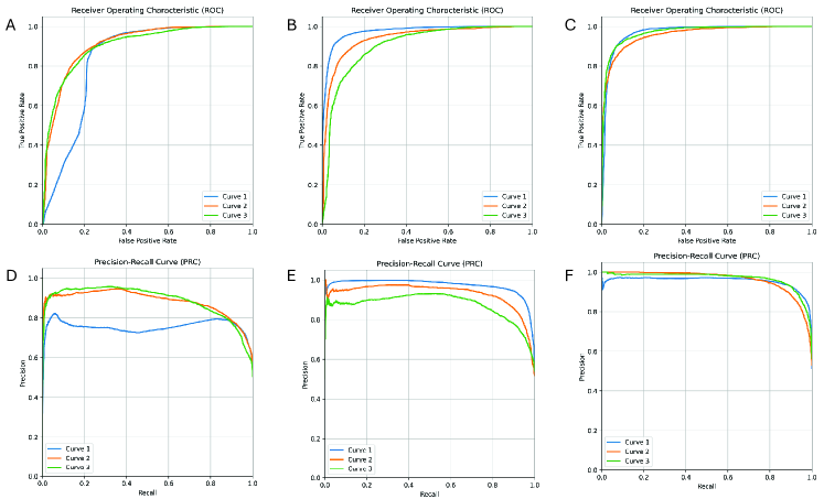
The figures reveal that the model rapidly ascends to nearly perfect true positive rates on the ROC curve while maintaining a low false positive rate, indicating its high effectiveness in distinguishing non-interactions between chemicals and genes. In the PRC curve, the model also displays precision and recall rates that exceed those of these two single-link prediction models, especially maintaining high precision at high recall levels, indicating the model’s significant advantage in ensuring the credibility of the prediction results. Overall, these graphs confirm the good performance of our model in prediction tasks.
2.3 Conflicting Edge Sampling Strategy
In our study, “edge conflicts” specifically refer to the conflicts during polarity predictions by the model, such as the same sample being predicted as both “activation” and “inhibition”. To avoid such conflicts, the model has to accurately distinguish between polar edges, such as activation and inhibition, which is crucial for understanding and predicting network behavior. By introducing the Cannot-Link (CL) conflicting edge sampling strategy, our model demonstrates enhanced discriminative capabilities when handling data with polar edges, significantly improving the accuracy in identifying polar relationships.
Although AUC and AP@k provide global view of model performances, they ignore the local intricacy when evaluating heterogenous networks. In our experiments, we explored the impact of the CL conflicting edge sampling strategy when classifying Must-Link (ML)-CL relationships using the RGCNTDDecoder model. Specifically, when applying the CL sampling strategy (YES), the AUROC value reached 0.959, the AUPRC value was 0.945, AP@20 was 0.902. In contrast, without using the CL sampling strategy (NO), the AUROC and AUPRC values were slightly higher, at 0.987 and 0.988 respectively, with AP@20 at 0.986. Further, considering the two new metrics we designed to evaluate the ability of handling polar relations, after using the CL sampling, the increased from 0.378 to 0.696 and the CP@500 also shown a considerable improvement from 0.766 to 0.862. Both metrics demonstrated that the model acquired the capability to distinguish polar relationships (Table 3). This indicates that although the CL sampling strategy may slightly reduce performance on some traditional metrics, it significantly lowers the probability of prediction conflicts when dealing with data of polar relations.
| CL sampling | |||||
|---|---|---|---|---|---|
| YES | 0.985 | 0.985 | 1.000 | 0.696 | 0.862 |
| NO | 0.966 | 0.962 | 0.978 | 0.378 | 0.766 |
| \botrule |
After constructing and evaluating multiple candidate models, we selected the best-performing model for further performance assessment. Our goal was to verify the model’s capability in predicting interactions between chemicals and genes and to understand the impact of different network connectivity on prediction accuracy. The best model’s ROC and PRC curves are shown in the figures (Fig. 2 A, D). In the Receiver Operating Characteristic (ROC) curves, the three lines illustrate the relationship between the true positive rate and the false positive rate at various thresholds. All three lines rapidly ascend to high true positive levels, indicating the model’s high sensitivity to positive cases. Especially, Curve 3 shows the steepest ascent before an increase in false positive rate, indicating its superior discriminative ability. The Precision-Recall (PRC) curves describe the relationship between precision and recall. Here, the closer a curve is to the upper right corner of the graph, the better the model’s performance. All curves maintain high precision at high recall rates, indicating the model’s ability to maintain high precision while keeping a high recall rate.
Additionally, we conducted tests on models employing the CL sampling strategy and those not utilizing any sampling strategy (hereafter referred to as the CL model and the No CL model, respectively) to observe their ability to identify different relational dynamics, particularly in distinguishing edges of opposite polarity. Using a test set of the same data volume, we predicted the probability of four types of relationships (Increase, Decrease, Binding, Affect) for each edge within the model. Notably, Increase and Decrease were considered relations of opposite polarity; the emergence of high probabilities simultaneously in both directions indicated a polarity conflict error, suggesting the model’s inability to differentiate edge polarity in the chemical-gene interactions.

For models before and after the implementation of the CL sampling strategy, we defined the Polarity Degree (C) as the absolute difference between the predicted probabilities of the ”Increase” and ”Decrease” directions for the same edge. We calculated the C values for both models and showed the frequency distribution of C values using histograms (Fig.2 E) and use Equation(12) to make transformation. It was observed that the model without the CL sampling strategy (represented in red) predominantly had a lower polarity degree, whereas the CL model (in blue) showed a higher polarity degree. This indicates that the CL model was more effective in managing or reducing contradictions and could more distinctly differentiate edge polarity.
Further, we marked correctly identified polar relationships with a +1 and incorrect or unrecognizable polar relationships with a -1 during the testing phase, depicted in red and blue lines, respectively. Through aggregate analysis of each line in the testing process (Fig.2 F), it was evident that in the CL model, occurrences and the extent of blue lines were significantly less frequent, indicating that instances of wrong predictions or errors were substantially fewer compared to the No CL model.
To validate the significant effect of our model on handling polar edges after employing the CL sampling strategy, we conducted a validation prediction on the model. We tested the model without the CL sampling strategy and with the CL sampling strategy on a randomly selected set of compounds, ranking the probability of each gene node across all connection scenarios. We separately tallied the top 100 nodes with the highest rankings in the polar relations of ”Increase” and ”Decrease”, converted the ranking values to log2, and plotted the log2-transformed rankings for each gene for increase and decrease scenarios (Fig.3 A-D). We sampled 900 compounds for repeated testing and plotted a boxplot of the average value of the log2 difference of the rankings of the top 100 nodes for each compound (Fig.3 E).

From the figures, it’s evident that in the absence of CL sampling (NO_CL), both the top 100 rankings for increase and decrease show little difference in log2 rank values, and overlap exists. However, after applying CL sampling, the overlap significantly reduces and disappears. Looking at the slope boxplots obtained through repeated testing, after applying CL sampling (CL), the slope values of the boxplots significantly increase, indicating that the ranking changes between the ”Increase” and ”Decrease” states of gene activity are more pronounced. The increase in slope values, especially the higher absolute values observed in the CL boxplot, clearly demonstrates that CL sampling enhances the differentiation between data points, making the distinction clearer in the direction of chemical-gene activity. Overall, CL sampling significantly enhances the differentiation effect of chemical-gene interaction data, which is crucial for understanding and interpreting gene regulatory mechanisms.
2.4 Impact of Network Component
As detailed in previous sections, our prediction model and its unique features, including the sampling method and decoder structure we adopted, have been discussed. Specifically, when we attempted to introduce subgraph structures (only chemical-chemical subgraph, only gene-gene subgraph, and both subgraphs) for training to explore their potential impact on the predictive performance of chemical-gene data, the results could have met our expectations. We discovered that, in some instances, adding subgraph structures could actually have a detrimental effect on model performance. Specifically, without using subgraphs, our model’s AUROC, AUPRC, and AP@20 evaluation metrics scored 0.985, 0.985, and 1.00000, respectively. And our two new mertics shown 0.695 and 0.121. However, upon introducing subgraph structures, these metrics experienced a decline (Table 4), indicating that in our model, subgraph structures are not a beneficial addition for enhancing predictive performance and might instead lead to performance degradation due to overcomplexity. This finding poses important considerations for model design: even if specific approaches are effective in other models or datasets, they may not be universally applicable.
| Prediction | |||||
|---|---|---|---|---|---|
| Subgraph | 0.839 | 0.825 | 0.781 | 0.521 | 0.771 |
| Only Chemical | 0.948 | 0.938 | 0.836 | 0.546 | 0.972 |
| Only Gene | 0.917 | 0.882 | 0.697 | 0.557 | 0.810 |
| No Subgraph | 0.985 | 0.984 | 1.000 | 0.695 | 0.866 |
| \botrule |
This result highlights the independence and efficiency of our model in processing chemical-gene interaction data. It indicates that for the specific dataset, our model has been optimized to a point where introducing subgraph structures not only fails to enhance predictive performance but may even reduce it due to the introduction of unnecessary complexity. Our study underscores the importance of developing models tailored to a dataset’s specific needs and provides practical guidance on balancing increasing model complexity with maintaining or enhancing performance. Future work will be needed to further explore the relationship between model complexity and predictive performance, as well as how to adjust the model structure for chemical-gene datasets to maximize prediction accuracy.
3 Method
3.1 Model Construction
Our model aims to compute the probability of the types of edges of interest given a specific node combination. This model employs an encoder-decoder architecture, where the encoder adopts the Graph Convolutional Network (GCN) principles designed by Yang et al. in the development of BioNet[23], and the decoder utilizes the design of Relational Graph Convolutional Networks (RGCN). During training, a strategy of sampling conflicting edges from signed and unsigned network combinations is adopted to address the diversity of edge types. Our model consists of two main components: GCNEncoder and RGCNTDDecoder. The GCNEncoder is divided into two layers; the first layer uses a graph convolutional layer to capture the features of the original input data; the second layer continues to abstract these features through another graph convolutional layer to form a more refined representation of the nodes. Subsequently, the RGCNTDDecoder combines Relational Graph Convolutional Network (RGCN) layers with the DEDICOM tensor decomposition layer, where the former is responsible for aggregating information according to different relation types, and the latter for parsing global and local interactions, ultimately generating predictions on the interactions between entities. The model’s architecture is shown in (Fig.4), which fully considers the multi-relational nature of graph data, enabling the capture of rich structural information and thereby holding extensive application potential in fields such as bioinformatics and recommendation systems.

3.1.1 Graph Convolutional Encoder
In this study, we employed a Graph Convolutional Encoder designed to capture and encode the intricate cooperative interactions between chemicals and genes. The graph convolutional encoder utilizes a hierarchical graph convolutional network architecture that iteratively aggregates and propagates information across nodes to learn node embeddings. The input to this architecture is a graph constructed from nodes represented as one-hot vectors and edges represented through adjacency matrices. In our work, we opt for a two-layer GCN optimized using Chebyshev polynomials, which has proven to exhibit enhanced performance, as evidenced in previous studies. The feature update for a node is given by Equation(1):
| (1) |
Here, represents a non-linear activation function, denotes the neighbors of node with a link type , and signifies the learnable parameter matrix associated with relation type . This equation is responsible for updating node features by leveraging information from first-order neighbors across different relation types. Progressing to the subsequent stage, the hidden state for each node is computed within the dimensionality of , and this is output as the node embedding , with indicating a two-layer graph convolutional network. These node embeddings are then incorporated into a multi-relational subgraph , processed through a secondary two-layer graph convolutional network as shown in Equation(2) :
| (2) |
In this expression, represents the set of relation types in the second stage, are the neighbors of under relation , and is the layer-specific weight matrix corresponding to relation in the second layer. This framework enables the encoding of higher-order neighborhood information, thereby enriching the representation of node features for downstream tasks. In this study, we improved upon the graph convolutional network encoder used by Yang et al[17]. to better suit our training data. Unlike the multi-relational subgraph approach mentioned in the previous model for the advanced node embedding process, we opted for a more direct method(Equation 3) to integrate the node embeddings of chemicals and genes:
| (3) |
Here, represents the final node embedding, with and respectively denoting the original embeddings of chemicals and genes. We merge these two types of node embeddings through a simple vector concatenation operation , instead of the multi-subgraph structure mentioned in the previous model. This design choice is based on the characteristics and needs of our data, aiming to simplify the model structure while preserving key information. Our model utilizes the hierarchical structure of the graph convolutional network during the encoding phase, first calculating the embeddings for each type of node separately and then combining these embeddings through the concatenation operation. Such a structure allows the model to reduce computational complexity without sacrificing performance, enabling us to train on larger-scale data.
3.1.2 Relational Graph Convolutional Network Tensor Decomposition
In this study, we introduce the Relational Graph Convolutional Network Tensor Decomposition (RGCNTDDecoder) model, which adopts an innovative multidimensional relation decoding strategy based on a close integration of Relational Graph Convolutional Network (RGCN) and Tensor Decomposition (TD) techniques. This model, by superimposing a specially designed tensor decomposition layer on top of the graph convolutional layer, is able to capture and decode the complex relationships between entities more precisely. Our aim with this structural improvement is to enhance the model’s performance on multi-relational data prediction tasks. In the RGCNTDDecoder, we employ the following mathematical Equation(4) to express the improved tensor decomposition layer.
| (4) |
Here, represents the predicted relational score between entity and entity , denotes a non-linear activation function, and indicates the Hadamard product. and respectively represent the embeddings of the entities. Our RGCNTDDecoder takes the output of the RGCN layer as input for the tensor decomposition algorithm, using the graph structural features captured by the RGCN to enhance relation prediction. The update process of the RGCN layer is described by the following Equation(5):
| (5) |
denotes the entity embeddings at layer , is the total number of relation types, is the set of neighboring entities of entity under relation , is a normalization constant, is the weight matrix specific to the relation at layer , and is the embedding of entity at layer . Within the RGCNTDDecoder, we employ a joint optimization strategy to train both the RGCN layer and the tensor decomposition layer simultaneously. The loss function Equation(6) is defined as the cross-entropy loss for the prediction of inter-entity relations, combined with a regularization term to prevent overfitting:
| (6) |
Wherein, is the set of all entity pairs in the training set, is the true label of the relationship between entity pair , is the regularization parameter, and represents all parameters within the model. Through this joint optimization strategy, the model not only learns to extract effective feature representations from the graph structure, but also learns how to make accurate predictions of complex relationships through the tensor decomposition layer. This end-to-end training approach allows different parts of the model to interact and coordinate with each other, thereby improving the accuracy of predictions and the model’s generalization ability.
3.2 Network Construction
In this study, we constructed a network of interactions between compounds and genes for the training of graph neural networks. By delving into open-source databases, we generated a graph for graph neural network training using compound-gene records obtained from the STITCH database[20]. Considering exploring the actual significance of compounds and genes, we mapped the PubChem CID used by the STITCH database[24] to the CHEBI ID in the ChEBI database[25]. The ChEBI database excludes protein molecules encoded by genes and other insignificant small molecules, focusing only on chemically meaningful molecules. Moreover, ChEBI’s ontology provides a rich structure that enables researchers to understand the relationship between specific chemical entities and the broader chemical world[26]. Similarly, we mapped protein IDs used by the STITCH from the String database to the widely used NCBI Gene ID. After data cleaning and removing meaningless compound molecules, we obtained a heterogeneous Chemical-Gene graph containing 12,537 compound nodes, 28,432 gene nodes, and 183,3943 interaction records, existed four relations (Table 5).
| No. | Realtion Name | Number of the edges |
|---|---|---|
| 1 | Increase | 752,037 |
| 2 | Decrease | 667,187 |
| 3 | Binding | 403,915 |
| 4 | Affect | 10,803 |
| \botrule |
Furthermore, we introduced homogeneous graphs such as the Chemical-Chemical and Gene-Gene interaction networks. On the one hand, we aimed to provide the model with more information to enhance its predictive capability; on the other hand, we wanted to observe the impact of complex network information input on model performance. The Gene-Gene interaction network was derived from 1,307,492 interaction records from the String database[27]. Chemical-Chemical interaction data was obtained from 1,770,581 records in the CHEBI database[28].
3.3 Prediction of Compound-Gene Interactions
Usually chemical-gene links and gene-chemical links were predicted separately (Equation(7)).
| (7) |
where and , respectively, represent the constructed embeddings for compounds and genes, and and denote the parameters used for tensor decomposition. We combine these two predictions in the following (Equation8):
| (8) |
In our approach, by integrating predictions of chemical-gene and gene-chemical interactions, we aim to overcome biases that single-direction predictions might introduce and to enhance robustness against potential imbalances in the dataset. This fusion method not only improves the model’s generalization ability for complex interactions between chemicals and genes, but also enhances the overall accuracy of the predictions, as validated in our subsequent experiments.
3.4 Handling Polar Edges in Chemical-Gene Prediction Tasks
In the chemical-gene prediction task, our dataset presented the challenge of polar edges, where the pair of a chemical and a gene (e.g., Chem A-Gene B) might have signs of direction (i.e. increase, decrease) that are supposed to be mutually exclusive. To effectively handle these polar edges, we adopted a dual sampling strategy that includes ”Must-Link” (ML) and ”Cannot-Link” (CL) constraints[29]. This sampling strategy is defined as follows Equation(9):
| (9) | ||||
The modeling of these links is captured through a custom-designed loss function, which aims to maximize the score difference between and , penalizing the model for polarity predictions. The loss function Equation(10) is defined as follows, where represents the loss for a set of relationship types in the network:
| (10) |
Here, and represent the edges within the same set of relationship types , and denotes the scoring function that assigns prediction scores to edges based on model output. The loss function enhances separation by subtracting the score of from that of , adding a constant margin of 1 to ensure separation, and applying a hinge function to penalize only when the margin is not met. In our implementation, we specifically targeted the polarity information between the ”Increase” and ”Decrease” relationship types, enhancing the model’s ability to differentiate mutually exclusive interactions. By incorporating this mechanism into the training routine, our model learned more nuanced data representations that reflect the complex nature of biological systems, where some relationships are inherently contradictory. This approach has been proven to improve the model’s discriminative ability, leading to more accurate and biologically reasonable predictions
3.5 Metrics Design
In this study, we introduced a variety of evaluation metrics to assess our model, in addition to the Area Under the Receiver Operating Characteristic Curve (AUROC) and Area Under the Precision-Recall Curve (AUPRC), as well as AP@20. We have also designed two new metrics specifically focused on the model’s ability to distinguish polar edges. These metrics not only demonstrate the performance of our model in predicting chemical-gene interactions but also offer significant reference value for future related research.
3.5.1 Average Precision at Polar Edges
In this study, we introduce a new metric to assess the ability of predictive models to differentiate between the effects of chemicals on genes, specifically ”Increase” and ”Decrease” interactions. Specifically, is defined as the absolute difference between the probabilities of ”Increase” and ”Decrease” edges predicted by the model by the following Equation(11).
| (11) |
where and represent the model’s predicted probabilities of a chemical increasing or decreasing a gene’s activity, respectively. This metric allows us to quantify the model’s confidence and ability in distinguishing between these two types of interactions without altering the internal structure of the data. However, the initial distribution of values is typically long-tailed, indicating a certain level of uncertainty in the model’s predictions for these interactions.
To enhance the statistical properties of and make it more suitable for data analysis and interpretation, we applied a mathematical transformation. The chosen transformation function is monotonically increasing from 0 to 1, preserving the original ordering of values without altering their relative magnitudes. Additionally, this transformation employs the natural logarithm function () to standardize the range of . The logarithm effectively processes and compresses the high dynamic range of , resulting in a smoother and more uniform distribution. The function includes a scaling constant such as which could be replaced with other alternatives. The transformation function is specified as follows in Equation(12):
| (12) |
This function was chosen for several reasons: Firstly, by using a scaling factor, we enhance the function’s sensitivity to changes in , allowing for a greater distinction of mid-range values of after transformation. This more clearly reflects the model’s predictive capabilities at different levels. Secondly, the function ensures that the transformed values of always remain between 0 and 1, which is more intuitive for interpretation. Lastly, this transformation significantly improves the original long-tail distribution of , making the transformed more uniform, thus helping the visual inspections.

We observed significant changes in the distribution of before and after transformation. Prior to transformation(Fig.5 A), the distribution of exhibited a long-tailed shape, particularly in the non-CL model distribution, where a dense concentration of low values reflected substantial uncertainty in the model’s ability to distinguish between ’Increase’ and ’Decrease’ interactions. A long-tail distribution implies the frequent occurrence of extreme values, which can lead to instability in statistical analysis and reduced efficiency in model training.
After the mathematical transformation (Fig.5 B), the distribution of improved significantly, especially within the CL model. The transformed distribution of values is closer to a normal distribution, with reduced long-tail effects and enhanced symmetry and concentration of the distribution. The transformation of the metric was primarily implemented to facilitate easier interpretation of the model outputs. By adjusting to a more interpretable distribution, we enhance the clarity and usability of the metric in practical applications. This straightforward adjustment allows for a more intuitive understanding of the differences between ’Increase’ and ’Decrease’ interactions predicted by the model.
In summary, the purpose of this transformation is to simplify the interpretation process, making it more straightforward to apply and derive insights from the model. This approach ensures that the metric’s representation is easily understandable, which is crucial for effective decision-making in practical scenarios.
3.5.2 Polarity Degree (C)-based Precision
To comprehensively assess the model’s performance under conditions of high confidence in its predictions, we introduce the Polarity Degree (C)-based Precision at 500 (CP@500) metric. This metric evaluates the model’s accuracy in its top 500 most confident predictions, providing a measure of the model’s precision in high-confidence decisions.
Firstly, for each instance in the dataset, we calculate the absolute difference between the predicted probabilities by Equation(12). Subsequently, all predictions are sorted in descending order based on the value, ensuring that the predictions with the highest confidence (largest values) are prioritized at the top of the list.
Next, we compare the predicted category with the actual true category to determine the correctness of each prediction. A prediction is marked as correct (1) if the predicted category matches the true category; otherwise, it is marked incorrect (0). Based on this, the first k predictions from the sorted list are selected, and the number of correct predictions among these is calculated to compute CP@k by the following Equation(11):
| (13) |
By introducing CP@k, not only do we evaluate the model’s accuracy in making its most certain predictions, but we also highlight the model’s performance under high confidence. This metric provides an intuitive and effective way to compare different models’ performance in their most confident predictions, particularly suitable for applications in high-stakes decision-making scenarios.
3.5.3 AUC for polar edge
Furthermore, inspired by the AUC (Area Under the Curve) evaluation methodology, we have devised a new metric—Area Under the Curve for polar edge prediction (). This metric is specifically designed to accurately assess the performance of our model in predicting the polarity (activation or inhibition) relationships between nodes in a network, especially in dealing with uncertain or polarity information. To this end, we begin by randomly selecting pairs of nodes, where the connections are defined as edges with activation or inhibition polarity. The model’s task is to predict the probabilities of activation (’Increase’) and inhibition (’Decrease’) , and to determine the actual polarity of the edge based on these probabilities. We utilize a binary indicator , which is assigned a value of 1 when the model’s predicted probability of activation is higher than that of inhibition and the actual polarity is activation, or vice versa for inhibition. This allows us to measure the degree of consistency between the model’s predictions and the actual polarity. The metric is computed using the formula Equation(14):
| (14) |
where is the total number of samples, and calculates the sign of the difference in the predicted probabilities.
Our metric is particularly applicable to biological network analysis, sensitively reflecting the model’s ability to discern polar edges—especially the ambiguous or polarity signals common in complex biological data. Compared to traditional metrics, offers a more precise and comprehensive standard of measurement, enabling researchers to gain deeper insights into and improve the model’s performance in bioinformatics applications.
4 Conclusion
Our proposed model employs a joint optimization strategy, featuring a decoder that combines Relational Graph Convolutional Network (RGCN) with Tensor Decomposition (TD), named RGCNTDDecoder. This approach aims to train the relational graph convolutional network layer and tensor decomposition layer simultaneously, focusing on improving the model’s performance on multi-relational data prediction tasks. By integrating chemical-gene and gene-chemical predictions, and employing a dual sampling strategy for polar edges, our approach overcomes biases that may be introduced by single-direction predictions, resolves contradictory prediction issues, and enhances the model’s robustness against potential imbalances in the dataset. We also introduced two novel evaluation metrics specifically designed to address the issue of polarity edges in the model. These metrics effectively assess the model’s capability to distinguish polarity edges, providing a quantitative measure of its ability to perceive edges with conflicting relationships. The implementation of these metrics could inspire and inform future research in this area, enhancing the understanding and development of models that accurately identify and handle polarity edges. Experimental results demonstrate that our model exhibits outstanding performance in predicting interactions between genes and chemicals, especially showing robustness in handling class imbalance and label noise. Furthermore, we demonstrated that models focusing on single subgraphs can more effectively capture and understand the relationship dynamics within complex biological networks. By simplifying the model structure and reducing reliance on multiple subgraphs, our model not only lowers computational complexity but also improves training efficiency and performance on large-scale data.
In summary, our work not only provides new perspectives and tools for drug repurposing research but also, through innovative improvements to deep graph models, expands the possibilities of biomedical network analysis. These innovative approaches are expected to accelerate the drug discovery and repurposing process, bringing more and higher quality treatment options to patients, showcasing the unique advantages of our model in performance optimization on single subgraphs.
5 Authors’ Contribution
Conceptualization: Lun Yu, Mengji Zhang, Meijie Wang; Methodology: Mengji Zhang, Shuyi Jin, Lun Yu; Writing - original draft preparation: Shuyi Jin, Lun Yu; Writing - review and editing: Lun Yu, Meijie Wang
6 Conflicts of Interest
Authors declare that they have no conflict of interest.
7 Ethics Statement
This study does not contain any studies with human participants or animals performed by any of the authors.
8 Data and Code Availability Statement
The dataset and code used in this study are available from the corresponding author upon reasonable request.
References
- \bibcommenthead
- Pushpakom et al. [2019] Pushpakom, S., Iorio, F., Eyers, P.A., Escott, K.J., Hopper, S., Wells, A., Doig, A., Guilliams, T., Latimer, J., McNamee, C., et al.: Drug repurposing: progress, challenges and recommendations. Nature reviews Drug discovery 18(1), 41–58 (2019)
- Abdulaziz et al. [2022] Abdulaziz, L., Elhadi, E., Abdallah, E.A., Alnoor, F.A., Yousef, B.A.: Antiviral activity of approved antibacterial, antifungal, antiprotozoal and anthelmintic drugs: Chances for drug repurposing for antiviral drug discovery. Journal of experimental pharmacology, 97–115 (2022)
- Ali et al. [2012] Ali, I., A Wani, W., Saleem, K., Haque, A.: Thalidomide: A banned drug resurged into future anticancer drug. Current drug therapy 7(1), 13–23 (2012)
- de Anda-Jáuregui et al. [2018] Anda-Jáuregui, G., Guo, K., McGregor, B.A., Hur, J.: Exploration of the anti-inflammatory drug space through network pharmacology: applications for drug repurposing. Frontiers in Physiology 9, 309929 (2018)
- Hopkins [2008] Hopkins, A.L.: Network pharmacology: the next paradigm in drug discovery. Nature chemical biology 4(11), 682–690 (2008)
- Zimmermann et al. [2007] Zimmermann, G.R., Lehar, J., Keith, C.T.: Multi-target therapeutics: when the whole is greater than the sum of the parts. Drug discovery today 12(1-2), 34–42 (2007)
- Crichton et al. [2018] Crichton, G., Guo, Y., Pyysalo, S., Korhonen, A.: Neural networks for link prediction in realistic biomedical graphs: a multi-dimensional evaluation of graph embedding-based approaches. BMC bioinformatics 19, 1–11 (2018)
- Zemouri et al. [2019] Zemouri, R., Zerhouni, N., Racoceanu, D.: Deep learning in the biomedical applications: Recent and future status. Applied Sciences 9(8), 1526 (2019)
- Sosa et al. [2019] Sosa, D.N., Derry, A., Guo, M., Wei, E., Brinton, C., Altman, R.B.: A literature-based knowledge graph embedding method for identifying drug repurposing opportunities in rare diseases. In: Pacific Symposium on Biocomputing 2020, pp. 463–474 (2019). World Scientific
- Gaudelet et al. [2021] Gaudelet, T., Day, B., Jamasb, A.R., Soman, J., Regep, C., Liu, G., Hayter, J.B., Vickers, R., Roberts, C., Tang, J., et al.: Utilizing graph machine learning within drug discovery and development. Briefings in bioinformatics 22(6), 159 (2021)
- Zitnik et al. [2018] Zitnik, M., Agrawal, M., Leskovec, J.: Modeling polypharmacy side effects with graph convolutional networks. Bioinformatics 34(13), 457–466 (2018)
- Cotto et al. [2018] Cotto, K.C., Wagner, A.H., Feng, Y.-Y., Kiwala, S., Coffman, A.C., Spies, G., Wollam, A., Spies, N.C., Griffith, O.L., Griffith, M.: Dgidb 3.0: a redesign and expansion of the drug–gene interaction database. Nucleic acids research 46(D1), 1068–1073 (2018)
- Du et al. [2018] Du, M., Ma, B., Meng, D.: Edge convergence problems on signed networks. IEEE transactions on cybernetics 49(11), 4029–4041 (2018)
- Derr et al. [2018] Derr, T., Ma, Y., Tang, J.: Signed graph convolutional networks. In: 2018 IEEE International Conference on Data Mining (ICDM), pp. 929–934 (2018). IEEE
- Yang et al. [2020] Yang, F., Fan, K., Song, D., Lin, H.: Graph-based prediction of protein-protein interactions with attributed signed graph embedding. BMC bioinformatics 21, 1–16 (2020)
- Mason et al. [2009] Mason, M.J., Fan, G., Plath, K., Zhou, Q., Horvath, S.: Signed weighted gene co-expression network analysis of transcriptional regulation in murine embryonic stem cells. BMC genomics 10, 1–25 (2009)
- Yang et al. [2020] Yang, F., Fan, K., Song, D., Lin, H.: Graph-based prediction of protein-protein interactions with attributed signed graph embedding. BMC bioinformatics 21, 1–16 (2020)
- Chen et al. [2022] Chen, M., Jiang, W., Pan, Y., Dai, J., Lei, Y., Ji, C.: Sgfnns: Signed graph filtering-based neural networks for predicting drug–drug interactions. Journal of Computational Biology 29(10), 1104–1116 (2022)
- Broido and Clauset [2019] Broido, A.D., Clauset, A.: Scale-free networks are rare. Nature communications 10(1), 1017 (2019)
- Kuhn et al. [2007] Kuhn, M., Mering, C., Campillos, M., Jensen, L.J., Bork, P.: Stitch: interaction networks of chemicals and proteins. Nucleic acids research 36(suppl_1), 684–688 (2007)
- Li et al. [2023] Li, Y., Xiong, H., Kong, L., Wang, S., Sun, Z., Chen, H., Chen, G., Yin, D.: Ltrgcn: Large-scale graph convolutional networks-based learning to rank for web search. In: Joint European Conference on Machine Learning and Knowledge Discovery in Databases, pp. 635–651 (2023). Springer
- Zhang et al. [2020] Zhang, Z., Li, M., Lin, X., Wang, Y.: Network-wide traffic flow estimation with insufficient volume detection and crowdsourcing data. Transportation Research Part C: Emerging Technologies 121, 102870 (2020)
- Yang et al. [2022] Yang, X., Wang, W., Ma, J.-L., Qiu, Y.-L., Lu, K., Cao, D.-S., Wu, C.-K.: Bionet: a large-scale and heterogeneous biological network model for interaction prediction with graph convolution. Briefings in bioinformatics 23(1), 491 (2022)
- Wang et al. [2009] Wang, Y., Xiao, J., Suzek, T.O., Zhang, J., Wang, J., Bryant, S.H.: Pubchem: a public information system for analyzing bioactivities of small molecules. Nucleic acids research 37(suppl_2), 623–633 (2009)
- Degtyarenko et al. [2007] Degtyarenko, K., De Matos, P., Ennis, M., Hastings, J., Zbinden, M., McNaught, A., Alcántara, R., Darsow, M., Guedj, M., Ashburner, M.: Chebi: a database and ontology for chemical entities of biological interest. Nucleic acids research 36(suppl_1), 344–350 (2007)
- Coudert et al. [2023] Coudert, E., Gehant, S., Castro, E., Pozzato, M., Baratin, D., Neto, T., Sigrist, C.J., Redaschi, N., Bridge, A.: Annotation of biologically relevant ligands in uniprotkb using chebi. Bioinformatics 39(1), 793 (2023)
- Mering et al. [2003] Mering, C.v., Huynen, M., Jaeggi, D., Schmidt, S., Bork, P., Snel, B.: String: a database of predicted functional associations between proteins. Nucleic acids research 31(1), 258–261 (2003)
- Zhang et al. [2020] Zhang, Z., Li, M., Lin, X., Wang, Y.: Network-wide traffic flow estimation with insufficient volume detection and crowdsourcing data. Transportation Research Part C: Emerging Technologies 121, 102870 (2020)
- Cheng et al. [2014] Cheng, J., Leng, M., Li, L., Zhou, H., Chen, X.: Active semi-supervised community detection based on must-link and cannot-link constraints. PloS one 9(10), 110088 (2014)