A data-driven Reconstruction of Horndeski gravity via the Gaussian processes

The GP regression is a powerful tool that merges the idea of a kernel and Bayesian analysis to make meaningful predictions of a function $H$ from a given data set $\{\left(z,H(z)\right)\}$ [75, 76]. Most notably, it is a non-parametric way of learning a function and so is a refreshing change of view in making cosmological predictions usually based on arbitrary parametrizations and Markov chain Monte Carlo (MCMC) methods [43, 44, 45]. In light of the existing tensions between early, i.e., during last scattering, and local cosmological observations, GP has also naturally emerged as a go-to approach in cosmology and is increasingly becoming a popular tool to make cosmological predictions without assuming a particular model of cosmology [44, 52, 46, 43, 45, 53, 54, 55, 56, 57, 58, 60, 61, 62, 77, 47, 78, 79, 80, 48, 49, 81, 82, 51].

Consider an observation $\{\left(z,H(z)\right)\}$ with uncertainties captured by the covariance matrix $C$. In order to reconstruct the function $H(z^{*})$ at the coordinates $z^{*}$ via the GP, we first assume a kernel $K\left(z^{*},\tilde{z}^{*}\right)$ that relates the function values at different coordinates $z^{*}$ and $\tilde{z}^{*}$ in the data set of observations. In terms of this kernel, the mean and the covariance of the GP reconstruction of the $n$th derivative of $H(z)$ at $z^{*}$ are given by

$$\langle H^{*(n)}\rangle=K^{(n,0)}\left(z^{*},Z\right)\left[K\left(Z,Z\right)+C\right]^{-1}H\left(Z\right)\,,$$

(3.1)

and

$$\text{cov}\left(H^{*(n)}\right)=K^{(n,n)}\left(z^{*},z^{*}\right)-K^{(n,0)}\left(z^{*},Z\right)\left[K\left(Z,Z\right)+C\right]^{-1}K^{(0,n)}\left(Z,z^{*}\right)\,,$$

(3.2)

respectively, where $Z$ stands for the union of the redshifts of the measurements and $y^{(n,m)}$ refers to the $n$th derivative of a function $y$ with respect to its first argument and the $m$th derivative with respect to the second argument. This kernel depends on hyperparameters that will be trained using a Bayesian implementation in order to fit the observations. However, in contrast with parametric approaches, the hyperparameters do not specify the shape of the function, but rather, they describe its characteristic scales in the $z$ and $H$ directions, typically, as a length scale $l$ and an amplitude $A$. In particular, we consider the simplest, infinitely-differentiable, and arguably the most widely-used kernel in machine learning, known as the radial basis function (RBF), also often referred to as the squared exponential kernel,

$$K\left(z,\tilde{z}\right)=A\exp\left(-\dfrac{\left(z-\tilde{z}\right)^{2}}{2l^{2}}\right)\,.$$

(3.3)

The hyperparameters $\left(l,A\right)$ are then selected by optimizing, or more consistently, marginalizing over the marginal likelihood $\mathcal{L}=p\left(H|Z,l,A\right)$. However, marginalization over the hyperparameters usually demands more computational power and can be impractically time consuming. Fortunately, in cosmology, and other applications, where the $\mathcal{L}$s are at least approximately Gaussian, optimization usually turns out to be a good approximation. In what follows, we will optimize over the hyperparameters to reconstruct the local Hubble function.

Two remarks are in order. First, the GP mean function is kept to zero in our reconstructions. This seems reasonable as we intend to obtain function values in regions encompassing the domain of the data points. Most importantly, this is in line with a data-driven, model-independent approach which would otherwise be compromised with, for example, a $\Lambda$CDM or another mean function. Second, it is often the case in GP applications that the reconstruction is tested for various kernels which lead to redundant results. For this reason, we pursue this work with only the most natural GP kernel (3.3), and instead investigate in detail the consequences of the choice of the kernel in a different paper [83] where we show that the reconstructions of the Hubble function per kernel can be at most in mild statistical tension with each other.

Our implementation is based on the public codes GaPP [43] and scikit [84] for the GP and cobaya [85] and getdist [86] for calibration of the absolute magnitude $M$ via MCMC to be described shortly. The codes used in this paper also used $numpy$ [87], $scipy$ [88], $seaborn$ [89], and $matplotlib$ [90]. A friendly implementation of the computations in this work is communicated as a two-part jupyter notebook [91] which can be freely downloaded [92].

We now apply the GP approach using the RBF kernel in Eq. (3.3) to a number of combined Hubble data sources, which we use to reconstruct the $H(z)$ data. This is done using three core sources of $H(z)$ data, namely cosmic chronometers (CC), supernovae of Type Ia (SNe) and baryonic acoustic oscillation (BAO). In addition, we consider three priors on $H(z)$ that have been reported in the literature, namely the Riess prior which is $H_{0}^{\rm R19}=74.03\pm 1.42\,{\rm km\,s}^{-1}{\rm Mpc}^{-1}$ [15], the Carnegie-Chicago Hubble prior $H_{0}^{\rm TRGB}=69.8\pm 1.9\,{\rm km\,s}^{-1}{\rm Mpc}^{-1}$ [93], and the latest value from the Planck collaboration (P18) $H_{0}^{\rm P18}=67.4\pm 0.5\,{\rm km\,s}^{-1}{\rm Mpc}^{-1}$ ($\Omega_{m0}=0.3153\pm 0.0073$ and $\Omega_{\Lambda}=0.6847\pm 0.073$) [13]. These $H_{0}$ priors clearly represent the current Hubble tension and are considered in this analysis to shed more light to this intriguing puzzle.

Adding some background on these priors, the $H_{0}^{\rm P18}$ estimates is the result of using (flat) $\Lambda$CDM as a fiducial model and cosmic microwave background (CMB) data from the Planck mission to predict the late time value of $H_{0}$ [13]. This contrasts with the cosmology independent estimates that come from local observations, where $H_{0}^{\rm R19}$ is the highest of these values and comes from long period observations of Cepheids in the Large Magellanic Cloud using the Hubble Space Telescope which significantly reduces the uncertainty in the measurement of $H_{0}$. We also consider measurements of the tip of the red giant branch (TRGB) where this turning point is used as a standard candle to predict values of $H_{0}^{\rm TRGB}$. While other prior values exist in the literature, these adequately represent the tension in the value of the Hubble constant.

On the data sets themselves, the CC data comprise the majority of the combined data set points with 29 (our of 40) points within the $z\lesssim 2$ range, and do not rely on any cosmological models [94, 95, 96, 97, 98]. For the SNe data set, we employ both the full Pantheon data set [99] and the compressed Pantheon compilation together with the CANDELS and CLASH Multi-cycle Treasury (MCT) data [100]. This is done using the corresponding covariance matrix, and where only five of the six points in Ref. [100] are used since the sixth point is non-Gaussian. In particular, we incorporate the compressed SNe data in the analysis by promoting the $E(z)$ data points to $H(z)=H_{0}E(z)$ using the $H_{0}$ priors and then feeding resulting $H(z)$ and the corresponding covariance matrix into the GP regression.

CC data depends on a differential ages technique between galaxies while the SNe data is compiled using Cepheid calibrated distance measurements for SNe event. Finally, we consider the BAO data from BOSS and eBOSS in Refs. [101, 102, 103, 104, 105, 106, 107, 108, 109]. While BAO data is not entirely independent from $\Lambda$CDM (due to the assumption of a fiducial radius of the sound horizon $r_{s}=147.78\,\mathrm{Mpc}$), they add value to the analysis as being data that emanates from the growth of large scale structure which has a strong bearing on the value of $H_{0}$. In particular, these measurements are made in terms of the comoving distance $d_{M}(z)/r_{s}$ and $d_{H}(z)/r_{s}$, where

$$d_{M}(z)=(1+z)d_{A}(z)\,,$$

(3.4)

and

$$d_{H}(z)=c/H(z)\,,$$

(3.5)

in which the Hubble expansion can be determined. Instead of relying on the sound horizon radius $r_{s}$, which consequently depends on a cosmological model which in this case is $\Lambda$CDM, we calculate the ratio $d_{M}(z)/d_{H}(z)$ from the BAO data set, cancelling out the dependence on $r_{s}$, and compliment this with a GP reconstructed angular-diameter distance $d_{A}(z)$ from the compressed Pantheon samples. This step assumes spatial-isotropy and the distance-duality relation, $d_{A}(z)=d_{L}(z)/(1+z)^{2}$, where $d_{A}(z)$ and $d_{L}(z)$ are the angular-diameter distance and luminosity distance, respectively, and also relies on a calibrated SNe absolute magnitude. Arguably, both spatial-isotropy and the distance-duality relation can be considered as cosmological assumptions, but neither requires any hard-parametrization like $\Lambda$CDM and, most importantly, both assumptions can be supported just as well with any metric theories of gravity.

Now, the full Pantheon data set was also considered where a cosmological model is necessary to obtain the Hubble data and thus calibrate the absolute magnitude $M$. Nonetheless, this quantity is related to the intrinsic brightness of a luminous object and so should not reflect, or at least, weakly reflect, the dynamics of cosmic expansion. This assertion is strongly supported by the fact that $M$ can be calibrated, provided an $H_{0}$ prior, with subpercent precision even when considering only the $z<0.1$ redshifts (the first 11 of 40 points) in the compressed Pantheon samples [99]. The calibrated $M$ which will be used later for the GP reconstruction of $H(z)$ per $H_{0}$ prior is shown in Fig. 1.

The mean and standard deviations are $M=-19.25\pm 0.05,-19.38\pm 0.06$, and $-19.45\pm 0.03$ for the R19, TRGB, and P18 $H_{0}$ priors, respectively. Lastly, the GP reconstructed Pantheon SNe apparent magnitudes is presented in Fig. 2.

We emphasize that the remarkable precision of this GP reconstruction of $m(z)$, achieved by performing the GP in $\log(z)$ (due to the drastic variance in the density of points across $z$), justifies and completes the outlined sound horizon-free construction of $H(z)$ from BAO.

In the present study, we perform a number of GP analyses using a combination of prior values. GP is a non-parametric reconstruction implementation but it does depend on the kernel hyperparameters. Given the level of precision in the discrepancy in $H_{0}$, we consider the RBF kernel in order to reduce any fine differences between these estimations of $H_{0}$.

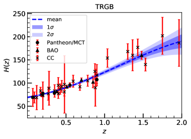
The reconstructed Hubble parameter is shown for the combined CC, Pantheon/MCT, and BAO data sets for each of the $H_{0}$ priors in Fig. 3. For completeness, we also write down the $\chi^{2}$ likelihoods for each of these reconstructions and the one for $\Lambda$CDM (taking in the P18 constraints [13]) in the subtitles of Fig. 3, and where

$$\chi^{2}=\sum_{i}\frac{\left(H_{\rm obs}(z_{i})-H_{\rm recon}(z_{i})\right)^{2}}{\sigma_{\rm obs}(z_{i})^{2}}\,,$$

(3.6)

for each data set in the combination. We do this to quantity possible over fitting which is a common pathology of non-parametric reconstruction methods. Indeed, this shows up in the $\chi^{2}$-statistics ($<40$, number of data points). Nonetheless, it can be seen that the constrained $\Lambda$CDM model based on the Planck 2018 release also overfits the joint data set. On the other hand, this overfitting by $\Lambda$CDM can in fact also be viewed as a remarkable coincidence considering that the Planck mission probes the physics of last scattering ($z\sim 1000$). The relative value of $\Delta\chi^{2}=\chi^{2}_{i}-\chi^{2}_{\Lambda\text{CDM}}$ may then be taken to provide a rough degree of how well a GP reconstruction fits the data.

In Fig. 3, we also notice that the low redshift behavior of the reconstructed Hubble diagram is not drastically different for the different prior selections. However, the uncertainties at high redshifts are impacted by this choice with R19 giving the largest uncertainties region. In fact, these reconstructions produce small uncertainty regions up to roughly $z\sim 1.5$ after which these regions start to grow due to the sparsity of observational data points in that region.

In the next section, the reconstructed $H(z)$ and its first derivative $H^{\prime}(z)$ will be used to predict Horndeski Lagrangian potentials. In doing so, it is important to highlight that $H(z)$ and $H^{\prime}(z)$ are naturally correlated together because of the GP reconstruction [43, 45]. That is, at each redshift $z^{*}$, this is fleshed out by the covariance matrix

$$\text{cov}\left(H(z^{*}),H^{\prime}(z^{*})\right)=K^{(0,1)}\left(z^{*},z^{*}\right)-K\left(z^{*},Z\right)\left[K\left(Z,Z\right)+C\right]^{-1}K^{(0,1)}\left(Z,z^{*}\right)\,.$$

(3.7)

To consistently obtain a function $f\left(H(z^{*}),H^{\prime}(z^{*}),\theta\right)$ where $\theta$ stands for any additional parameters, with a variance $\text{var}\left(\theta\right)$, we draw a large number of samples, a la Monte Carlo (MC), from the multivariate Gaussian distribution

$$\left(\begin{matrix}H\\ H^{\prime}\\ \theta\end{matrix}\right)\sim\mathcal{N}\left[\left(\begin{matrix}H\\ H^{\prime}\\ \theta\end{matrix}\right),\left(\begin{matrix}\text{cov}\left(H,H\right)&\text{cov}\left(H,H^{\prime}\right)&0\\ \text{cov}\left(H,H^{\prime}\right)&\text{cov}\left(H^{\prime},H^{\prime}\right)&0\\ 0&0&\text{var}\left(\theta\right)\end{matrix}\right)\right]\,,$$

(3.8)

and then take the mean, standard deviation, and other relevant statistical outputs of the resulting posterior distribution of the function $f$.

The simplest and perhaps most well-known potential construction method is in quintessence cosmology [69]. In this model, the Friedmann and scalar field equations are given by

$$3H^{2}=\rho+\dfrac{\dot{\phi}^{2}}{2}+V\left(\phi\right)\,,$$

(4.1)

$$2\dot{H}+3H^{2}=-P-\dfrac{\dot{\phi}^{2}}{2}+V\left(\phi\right)\,,$$

(4.2)

and

$$\ddot{\phi}+3H\dot{\phi}+V^{\prime}\left(\phi\right)=0\,,$$

(4.3)

respectively. It can of course be shown that Eq. (4.3) follows from Eqs. (4.1) and (4.2) as long as the perfect fluid’s energy is thermodynamically conserved. Using the Friedmann equations, it can then be shown that the potential and kinetic terms of the scalar field are given by

$$V\left(\phi\right)=\dot{H}+3H^{2}-\dfrac{\rho-P}{2}\,,$$

(4.4)

and

$$\dot{\phi}^{2}=-2\dot{H}-\left(\rho+P\right)\,.$$

(4.5)

Eq. (4.4) shows that the quintessence potential can be uniquely determined given a Hubble function and matter fields. The kinetic term $X=\dot{\phi}^{2}/2$ (through Eq. (4.5)) can be similarly obtained. We additionally assume non-relativistic matter fields which take on the P18 value for the current matter density parameter [13].

We can now use the GP reconstructed Hubble function to predict the shapes of the $V$ and $\phi^{\prime}(z)^{2}$, where $\dot{f}\left(t\right)=-(1+z)H(z)f^{\prime}(z)$ for an arbitrary function $f$ of time (or redshift). The results are shown in Fig. 4.

Note that by expressing the dimensionful quantities, in this case, $V$, in units of $H_{0}$, the tensions which exist at $z=0$ for the different $H_{0}$ priors can be alleviated in the construction. For example, in Fig. 4, the mean values of $V$ and $\phi^{\prime}(z)^{2}$ for any one of the priors always lie well within the $1\sigma$ contours of the two other priors. In this case, it can be seen that the potential and kinetic term traces out a particular shape regardless of the $H_{0}$ prior. This then constrains the quintessence potential. In principle, the explicit function $V\left(\phi\right)$ can also be obtained by integrating $\phi^{\prime}(z)$ to obtain $\phi$ up to a constant. However, we find that the mean $\phi^{\prime}(z)^{2}$ is mostly-negative throughout the late-time cosmological evolution. Notably, positive values of $\phi^{\prime}(z)^{2}$ which happen to occur near the upper $2\sigma$ contours can be used to predict $V\left(\phi\right)$. This should of course be taken with caution given that it hovers just around, and some times beyond, the $95\%$ confidence region. Nonetheless, the dark energy equation of state, $w_{\phi}=P_{\phi}/\rho_{\phi}$, can be obtained which in the quintessence model becomes

$$w_{\phi}=\dfrac{\dot{\phi}^{2}/2-V}{\dot{\phi}^{2}/2+V}\,.$$

(4.6)

However, instead of $w_{\phi}$ it turns out to be as convenient to additionally sample over the compactified variable $\arctan\left(1+w_{\phi}\right)$. We refer to this as a compactified dark energy equation of state. This alternative variable tames down the singularities which otherwise would make the MC procedure terribly unreliable, i.e., MC propagated errors in $w_{\phi}$ diverge at $z\sim 1$. The result of the additional sampling of the compactified dark energy equation of state is shown in Fig. 5.

In Fig. 5-(a), the median of the distribution and the $34.1\%$ of the probability mass surrounding it on both sides are shown. To see why this is a more consistent statistic, compared with the usual Gaussian-anchored mean $\pm$ $1\sigma$ statistic, we also show the resulting posterior distributions of $\arctan\left(1+w_{\phi}(z)\right)$ at different redshifts in Figs. 5-(b-d).

Clearly, for low redshifts, $z\lesssim 1$, the resulting distributions can be considered to be normally-distributed. However, at higher redshifts, it can be seen that the distribution not only starts to deviate away from normality, but even becomes bimodal and takes samples at $\arctan\left(1+w_{\phi}\right)\sim\pm\pi/2$ where $w_{\phi}$ diverges. For this reason, the median and the $34.1\%$ probability mass surrounding it from both sides can be considered as a more consistent statistic as it agrees with the mean $\pm$ $1\sigma$ when the distribution is normal, but it tracks the most concentration of probability mass even when the distribution is no longer normal. See Appendix A for a supplementary illustration of this point. In addition, a naive use of the mean $\pm$ $1\sigma$ statistic for a compactified variable may predict results outside of the domain of the compactified variable while the median $\pm$ $34\%$ probability mass will always only sample within this domain.

The results shown in Fig. 5 agree that dark energy may as well be vacuum energy, i.e., $w\approx-1$ or $\arctan\left(1+w_{\phi}\right)=0$, for low redshifts. On the other hand, the use of the compactified dark energy equation of state lets us understand a clearer picture of dark energy at earlier redshifts when the prediction of $w_{\phi}$ becomes spoiled by diverging uncertainties. For instance, at $z\gtrsim 1$, Figs. 5-(b-d) reveal that the onset of the divergence in the uncertainty of $w_{\phi}$ is alternatively due to the compactified variable starting take values with $|\arctan(x\sim\pm\pi/2)|\gg 1$. This sampling procedure on a compactified random will be utilized further to study dark energy in the two following Horndeski models.

To end this section, we recall that $\Omega_{m}$ is a free parameter which we fixed to its P18 value (anchored on $\Lambda$CDM) in order to avoid an otherwise ad hoc choice. The above reconstruction is therefore bias to this information. We briefly describe the reconstruction for other values of $\Omega_{m}$. Smaller $\Omega_{m}$ leads to higher $V(\phi)$ and $\phi^{\prime}(z)^{2}$, while larger $\Omega_{m}$ leads to lower $V(\phi)$ and $\phi^{\prime}(z)^{2}$. This can be also be deduced from Eqs. (4.4) and (4.5). In particular, for $\Omega_{m}\lesssim 0.1$, the reconstruction of $\phi^{\prime}(z)^{2}$ can be positive throughout. This can be taken to mean that quintessence and late-time data favor a smaller $\Omega_{m}$ than that of $\Lambda$CDM. We encourage the reader to test this out using our codes [92].

Another Horndeski construction method has been introduced recently in Ref. [73]. This is referred to as designer Horndeski (HDES) and is built on top of kinetic gravity braiding. To describe this method, we start with the cosmological field equations given by

$$3H^{2}=\rho-K(X)+2XK_{X}+3H\dot{\phi}^{2}G_{X}\,,$$

(4.7)

$$2\dot{H}+3H^{2}=-P-K(X)+2X\ddot{\phi}G_{X}\,,$$

(4.8)

and

$$\ddot{\phi}\left(-\dot{\phi}\left(3H\left(G_{XX}\dot{\phi}^{2}+2G_{X}\right)+K_{XX}\dot{\phi}\right)-K_{X}\right)-3\dot{\phi}\left(G_{X}\dot{H}\dot{\phi}+3G_{X}H^{2}\dot{\phi}+HK_{X}\right)=0\,,$$

(4.9)

where a subscript in the potentials $K(X)$ and $G(X)$ denote differentiation with respect to $X$. These are the Friedmann and scalar field equations. Also, a noteworthy feature in these shift symmetric models is that the scalar field equation can be written in the form

$$\dot{J}+3HJ=0\,,$$

(4.10)

where $J$ is the shift current given by

$$J=\dot{\phi}K_{X}+3H\dot{\phi}^{2}G_{X}\,.$$

(4.11)

Therefore, instead of the scalar field equation, one can consider as a surrogate the exact solution of Eq. (4.10), namely

$$\dot{\phi}K_{X}+3H\dot{\phi}^{2}G_{X}=\dfrac{\mathcal{J}}{a^{3}}\,,$$

(4.12)

where $\mathcal{J}$ is an integration constant which we refer to as a shift charge. The designer approach recognizes the constraint equations (Eqs. (4.7) and (4.12)) as two independent equations of the system but with three unknowns, i.e., $\left(H(a),K(X),G(X)\right)$. The system is then closed by a priori assuming $H(X)$. In this case, the exact solution of Eqs. (4.7) and (4.12) can be shown to be

$$K(X)=-3H_{0}^{2}\Omega_{\Lambda}+\dfrac{\mathcal{J}\sqrt{2X}H(X)^{2}}{H_{0}^{2}\Omega_{m0}}-\dfrac{\mathcal{J}\sqrt{2X}\Omega_{\Lambda}}{\Omega_{m0}}\,,$$

(4.13)

and

$$G_{X}(X)=-\dfrac{2\mathcal{J}H^{\prime}(X)}{3H_{0}^{2}\Omega_{m0}}\,.$$

(4.14)

Eqs. (4.13) and (4.14) fleshes out the designer approach. By complementing this with the GP, we can then make a predictive analysis of the $k$-essence and braiding potentials.

Before proceeding, we clarify that the designer Horndeski approach relies on a mapping between $X$ and $a$ which leads to a Horndeski theory $\left(K(X),G(X)\right)$. This then means that the designer trajectory $X_{\text{HDES}}(a)$ must not have fixed points. However, the resulting theory $\left(K(X),G(X)\right)$ may have other trajectories $X(a)$ and so in general fixed points are not prohibited in the designer approach.

As with Ref. [73], we take

$$X=\dfrac{c_{0}}{H(X)^{n}}\,,$$

(4.15)

where $c_{0}$ is a constant with units of $H_{0}^{n+2}$. Using the GP reconstructed Hubble function, we then obtain the predictions for $X$ and $H^{\prime}(X)$ shown in Fig. 6 for $n=1$ and $c_{0}=H_{0}^{n+2}$.

By expressing dimensionful physical quantities in units of the Hubble parameter $H_{0}$, we find that the mean $z=0$ prediction for each $H_{0}$ prior is always within the $1\sigma$ contours of the two other priors. This holds for both $X$ and $H^{\prime}(X)$ in Fig. 6 and, as we shall further see, also in the following figures. The precision of the $H_{0}$ prior also does play a role. In Fig. 6, the prediction using the Planck prior turns out to be the most stringent for all redshifts. Moving forward, Fig. 7 shows the predicted HDES potentials corresponding to Fig. 6 with $c_{0}=H_{0}^{n+2}$, $n=1$, and $\mathcal{J}/H_{0}=1$. In this analysis, we also assume the P18 cosmological parameter values.

Fig. 7 reveals the shape of the $k$-essence and braiding potentials. Most importantly, this shape appears to be consistent regardless of the choice of $H_{0}$ prior.

The dark energy equation of state can also be computed. In general, in shift symmetric kinetic gravity braiding, this is given by

$$w_{\phi}=\dfrac{-K+\sqrt{2X}\dot{X}G_{X}}{K-2X\left(K_{X}+3\sqrt{2X}H(X)G_{X}\right)}\,,$$

(4.16)

where the potentials $K$ and $G$ and their derivatives are evaluated at $X$. By substituting the HDES solution to Eq. (4.16), we obtain

$$w_{\phi}=-1+\dfrac{\mathcal{J}\sqrt{2X}\left(H(z)^{2}-H_{0}^{2}\Omega_{\Lambda}\right)}{3H_{0}^{4}\Omega_{m0}\Omega_{\Lambda}}-\dfrac{2\mathcal{J}\sqrt{2X}(1+z)H(z)H^{\prime}(z)}{9H_{0}^{4}\Omega_{m0}\Omega_{\Lambda}}\,.$$

(4.17)

Using the reconstructed Hubble function and its first derivative, we can therefore obtain the dark energy equation of state. This is shown in compactified version, like we did with the quintessence case, in Fig. 8.

Interestingly, the compactified dark energy equation of state here retains single-modality for all redshifts, unlike its quintessence counterpart. Above all, this result is showing a strong deviation from $\Lambda$CDM at higher redshifts. This is shown in Fig. 8(a) and is also revealed more closely in Figs. 8-(b-d). In particular, the posteriors of the probability distribution for the $z=1.5$ and $z=2$ cases for all $H_{0}$ priors are strongly concentrated outside of the $\Lambda$CDM limit ($\arctan\left(1+w_{\phi}\right)=0$). This may have been expected due to the $k$-essence and braiding potentials growing at higher redshifts (Figs. 7-(a) and (c)); nonetheless, this is worth highlighting as it points to potential future work with perturbations. Consider as an example the case of structure formation where the braiding potential may significantly affect.

To end the section, we recall that Fig. 8 shows the posterior of $\arctan\left(1+w_{\phi}(z)\right)$ and not $w(z)$. So while the error bands do indeed become smaller in $\arctan\left(1+w_{\phi}(z)\right)$ for high redshifts, the corresponding uncertainty in $w(z)$ in fact becomes larger. In particular, Figs. 8(b-d) show that the posterior for $z\sim 2$ is nearly localized at $\arctan\left(1+w(z)\right)\sim\pi/2$ which corresponds to very large mean values and uncertainties in $w(z)$. We clarify this further in Appendix A where the posterior of a random variable and its compactified version are displayed side by side.

Tailoring Horndeski [74] is related to both quintessence potential and HDES models and is amenable to this reconstruction method. This can be considered as the $J(t)=0$ limit of HDES but it works more similar with quintessence in the sense that one does not have to rely on an a priori $H(X)$ in order to single out a particular potential ¹¹1In Ref. [73], it was mentioned that the $J(t)=0$ limit of HDES is $\Lambda$CDM. This was based on naively making the shift charge $\mathcal{J}$ vanish in Eqs. (4.13) and (4.14). However, this limit should be merely realized to be just an artifact of the particular parametrization of the HDES solution (Eqs. (4.13) and (4.14)). In general, with $\mathcal{J}=0$, one should start again with Eqs. (4.7) and (4.12), from which HDES was derived. This will inevitably lead to the tailoring Horndeski approach..

The field equations of the theory are given by

$$3H^{2}=\rho+2\Lambda+\dfrac{\dot{\phi}^{2}}{2}+3H\dot{\phi}^{3}G_{X}\,,$$

(4.18)

$$2\dot{H}+3H^{2}=-P+2\Lambda-\dfrac{\dot{\phi}^{2}}{2}+G_{X}\dot{\phi}^{2}\ddot{\phi}\,,$$

(4.19)

and

$$\ddot{\phi}\left(-3H\left(G_{XX}\dot{\phi}^{3}+2G_{X}\dot{\phi}\right)-1\right)-3\dot{\phi}\left(G_{X}\dot{H}\dot{\phi}+3G_{X}H^{2}\dot{\phi}+H\right)=0\,.$$

(4.20)

Note that the above equations can be obtained from Eqs. (4.7), (4.8), and (4.9) by substituting $K(X)=X-2\Lambda$. The solution of the system will therefore also lie on the dynamical hypersurface determined by Eq. (4.12). In contrast, the tailoring Horndeski approach recognizes the $J(t)=0$ as a dynamical attractor and so builds the solution on top of this hypersurface. One can then write down

$$G_{X}(X)=-\dfrac{1}{3\sqrt{2X}H(X)}\,.$$

(4.21)

Since there is only one potential, i.e., $G_{X}$, Eq. (4.21) can be used to obtain model independent necessary conditions by substituting into Eqs. (4.18) and (4.19). The emerging necessary conditions are given by

$$X=3\left(H_{0}^{2}\Omega_{m}(z)+H_{0}^{2}\Omega_{\Lambda}-H^{2}\right)\,,$$

(4.22)

and

$$2\dot{H}+3H^{2}=-P+3H_{0}^{2}\Omega_{\Lambda}-X-\dfrac{\dot{X}}{3H}\,,$$

(4.23)

where $\Omega_{m}(z)=\rho(z)/\left(3H_{0}^{2}\right)$ and $\Omega_{\Lambda}=2\Lambda/\left(3H_{0}^{2}\right)$. The kinetic density can then be uniquely determined for a given Hubble function by using Eq. (4.22). Moreover, by eliminating $X$ in Eqs. (4.22) and (4.23), one can recover the thermodynamic conservation law

$$\dot{\rho}+3H\left(\rho+P\right)=0\,\$$

(4.24)

which ensures the consistency of the method. In summary, the braiding potential and the scalar field’s kinetic density can be uniquely assigned to a given Hubble function through Eqs. (4.21) and (4.22).

By complementing the above outlined tailoring Horndeski method with the GP reconstructed Hubble function, we now obtain predictions of the theory. The resulting kinetic density is shown in Fig. 9.

Here, we also consider the P18 cosmological parameter values, and so, once more, by expressing dimensionful quantities in units of $H_{0}$, we find consistent shapes of the predicted functions regardless of the choice of $H_{0}$ prior. It is noteworthy that the scalar field has spent most of its late-time dynamics with $|X/H_{0}^{2}|\ll 1$. This is important as the braiding potential (Eq. (4.21)) possesses a singularity at $X=0$ and so MC sampling over $G_{X}$ can be expected to result to posteriors with very large, consequently unreliable, uncertainties. Fig. 9 also shows that an appreciable size of the samples fall to the region $X<0$. This is problematic from a computational point of view when sampling $G_{X}$ because of the square root in Eq. (4.21). To avoid the above mentioned issues, we proceed by additionally sampling over a compactified, real, random variable, $\tilde{G}_{X}^{2}$ given by

$$\tilde{G}_{X}^{2}=\arctan\left(\dfrac{H_{0}^{4}}{18XH\left(X\right)^{2}}\right)\,.$$

(4.25)

We refer to this as a compactified braiding potential. The results are shown in Fig. 10.

Here, it is shown that $\tilde{G}_{X}^{2}$ may also accept negative values at low redshifts (or low $X$), whenever $X<0$ can be drawn with appreciable probability. In such cases, the braiding potential is going to be undefined, or rather that the model is disfavored by the data. However, at higher redshifts, the distribution tends to become more concentrated towards positive values. The inset of of Fig. 10-(a) proves this. As complementary to Fig. 10, snapshots of the posterior distribution of the distributions of $\tilde{G}_{X}^{2}$ at redshifts $z=0,0.5,1,1.5,2$ are shown in Fig. 11.

This shows that the distribution of $\tilde{G}_{X}^{2}$ is generally bimodal and supports the use of the median and its $34.1\%$ surrounding mass as a reasonable statistic. At $z=0$, Figs. 11-(a-c) show that $\tilde{G}_{X}^{2}$ may almost-equally be positive or negative and samples may even be drawn with appreciable probability near the boundaries, $\tilde{G}_{X}^{2}\sim\pm\pi/2$, of the random variable. Interestingly, at higher, or earlier, redshifts, the probability mass at negative $\tilde{G}_{X}^{2}$ always decreases with an increase in the redshift, i.e., the weight of the samples drawn at negative $\tilde{G}_{X}^{2}$ becomes smaller for increasing $z$. This is a consistent result throughout the $H_{0}$ priors and so suggests that the braiding may have played a relevant earlier minor role in cosmic history. Fig. 11-(d) supports this interpretation. Indeed, at $z=2$, the posteriors of $\tilde{G}_{X}^{2}$ can already be considered to be practically single-modal and undeniably heavier at $\tilde{G}_{X}^{2}>0$, where the braiding potential $G_{X}$ can be computed. A crude estimate of $H_{0}^{2}G_{X}$, based on Fig. 11-(d) and $\arctan\left(x\ll 1\right)\sim x$, leads to $H_{0}^{2}G_{X}\sim 0.1$ at $z\sim 2$.

The dark energy equation of state in tailoring Horndeski can also be computed using Eq. (4.16). Substituting $K(X)=X-2\Lambda$ and then using the tailored solution (Eqs. (4.21) and (4.22)), it is straightforward to obtain

$$w_{\phi}(z)=\dfrac{H(z)\left(3H(z)-2(1+z)H^{\prime}(z)\right)}{3\left(-H(z)^{2}+H_{0}^{2}\Omega_{m0}\left(1+z\right)^{3}\right)}\,.$$

(4.26)

This is notably the exact same expression that can be obtained by assuming that dark energy is a perfect fluid with an equation of state $w(z)$. The results of the sampling over the compactified dark energy equation of state is shown in Fig. 12.

It is most interesting to point out that this looks very similar to Fig. 12 even though the earlier analysis of quintessence did not take into account $\Omega_{\Lambda}$. Similar conclusions can therefore be drawn. First, at low redshifts, the posterior distributions of the compactified dark energy equation of state can be considered to be approximately Gaussian distributed. However, at higher redshifts, this cannot anymore be taken to be true as the distribution becomes bimodal and an appreciable fraction of samples fall too close to the boundaries $\sim\pm\pi/2$ of the compactified region. In particular, for $z=2$ in Figs. 12-(b-d), the probability mass appear to be mostly heavier at the positive side, i.e., $\arctan\left(1+w_{\phi}\right)\sim 1$, suggesting a deviation from $\Lambda$CDM. The implications of this should be further examined in a future work.

We now summarize the constraints on the dark energy equation of state at $z=0$ obtained in this work in Table 1.

The $w_{\text{DE}}\,(z=0)$ constraints from quintessence and tailoring Horndeski differ only in their fifth significant digit which is well within the predictability region that can be reasonably expected from the reconstruction method. For both of these theories, the dark energy equation of state remains consistent with each other and regardless of the $H_{0}$ prior. In this background the priors on the Hubble data have little to no impact on the equation of state reconstructions since these fine differences will be suppressed by the precise formula that expresses the quantity. The situation is entirely different for the direct reconstruction of the Hubble diagram where priors not only have a significant impact on the diagrams that are produced but also on the reconstructed values of $H_{0}$ which is one of the most important results from this reconstruction method.

On the other hand, the $w_{\text{DE}}(z=0)$ constraints coming from designer Horndeski should be taken more carefully as it strongly depends on the assumed shift charge $\mathcal{J}$ and so is not completely predictive with just the low-redshift data. Since the shift charge is a constant throughout the evolution, it would have been then highly coincidental if it scales with the Hubble parameter today. The shift charge can instead be constrained with the CMB as done in Ref. [73]. Alternatively, combining the low redshift observations from Hubble data and $f\sigma_{8}$ can be considered to constrain the shift charge.

It is also interesting to point out the recent work of Ref. [110] which suggests that quintessence is at odds with local determinations of $H_{0}$. Extending this perturbative analysis to broader Horndeski theories may lead to a better understanding of dark energy and the $H_{0}$ tension.

References

- [1] Supernova Search Team collaboration, Observational evidence from supernovae for an accelerating universe and a cosmological constant, Astron.J. 116 (1998) 1009 [astro-ph/9805201].
- [2] Supernova Cosmology Project collaboration, Measurements of Omega and Lambda from 42 high redshift supernovae, Astrophys.J. 517 (1999) 565 [astro-ph/9812133].
- [3] S. Dodelson, Modern Cosmology. Academic Press, 2003.
- [4] T. Clifton, P. G. Ferreira, A. Padilla and C. Skordis, Modified Gravity and Cosmology, Phys. Rept. 513 (2012) 1 [1106.2476].
- [5] S. Weinberg, The cosmological constant problem, Rev. Mod. Phys. 61 (1989) 1.
- [6] P. Bull et al., Beyond CDM: Problems, solutions, and the road ahead, Phys. Dark Univ. 12 (2016) 56 [1512.05356].
- [7] V. Sahni and A. A. Starobinsky, The Case for a positive cosmological Lambda term, Int. J. Mod. Phys. D 9 (2000) 373 [astro-ph/9904398].
- [8] V. Sahni and A. Starobinsky, Reconstructing Dark Energy, Int. J. Mod. Phys. D 15 (2006) 2105 [astro-ph/0610026].
- [9] E. J. Copeland, M. Sami and S. Tsujikawa, Dynamics of dark energy, Int. J. Mod. Phys. D15 (2006) 1753 [hep-th/0603057].
- [10] S. Capozziello and M. De Laurentis, Extended Theories of Gravity, Phys. Rept. 509 (2011) 167 [1108.6266].
- [11] E. Di Valentino et al., Cosmology Intertwined II: The Hubble Constant Tension, 2008.11284.
- [12] E. Di Valentino et al., Cosmology Intertwined III: and , 2008.11285.
- [13] Planck collaboration, Planck 2018 results. VI. Cosmological parameters, Astron. Astrophys. 641 (2020) A6 [1807.06209].
- [14] J. L. Bernal, L. Verde and A. G. Riess, The trouble with , JCAP 10 (2016) 019 [1607.05617].
- [15] A. G. Riess, S. Casertano, W. Yuan, L. M. Macri and D. Scolnic, Large Magellanic Cloud Cepheid Standards Provide a 1% Foundation for the Determination of the Hubble Constant and Stronger Evidence for Physics beyond CDM, Astrophys. J. 876 (2019) 85 [1903.07603].
- [16] K. C. Wong et al., H0LiCOW – XIII. A 2.4 per cent measurement of H0 from lensed quasars: 5.3 tension between early- and late-Universe probes, Mon. Not. Roy. Astron. Soc. 498 (2020) 1420 [1907.04869].
- [17] Planck collaboration, Planck 2015 results. xiii. cosmological parameters, Astron.Astrophys. 594 (2016) A13 [1502.01589].
- [18] A. G. Riess, The Expansion of the Universe is Faster than Expected, Nature Rev. Phys. 2 (2019) 10 [2001.03624].
- [19] D. W. Pesce et al., The Megamaser Cosmology Project. XIII. Combined Hubble constant constraints, Astrophys. J. Lett. 891 (2020) L1 [2001.09213].
- [20] T. de Jaeger, B. E. Stahl, W. Zheng, A. V. Filippenko, A. G. Riess and L. Galbany, A measurement of the Hubble constant from Type II supernovae, Mon. Not. Roy. Astron. Soc. 496 (2020) 3402 [2006.03412].
- [21] E. Di Valentino, A. Melchiorri and J. Silk, Planck evidence for a closed Universe and a possible crisis for cosmology, Nature Astron. 4 (2019) 196 [1911.02087].
- [22] W. Handley, Curvature tension: evidence for a closed universe, Phys. Rev. D 103 (2021) L041301 [1908.09139].
- [23] G. W. Horndeski, Second-order scalar-tensor field equations in a four-dimensional space, Int. J. Theor. Phys. 10 (1974) 363.
- [24] T. P. Sotiriou and V. Faraoni, f(R) Theories Of Gravity, Rev. Mod. Phys. 82 (2010) 451 [0805.1726].
- [25] A. De Felice and S. Tsujikawa, f(R) theories, Living Rev. Rel. 13 (2010) 3 [1002.4928].
- [26] S. Nojiri and S. D. Odintsov, Modified f(R) gravity consistent with realistic cosmology: From matter dominated epoch to dark energy universe, Phys. Rev. D 74 (2006) 086005 [hep-th/0608008].
- [27] W. Hu and I. Sawicki, Models of f(R) Cosmic Acceleration that Evade Solar-System Tests, Phys. Rev. D 76 (2007) 064004 [0705.1158].
- [28] S. A. Appleby and R. A. Battye, Do consistent models mimic General Relativity plus ?, Phys. Lett. B 654 (2007) 7 [0705.3199].
- [29] A. A. Starobinsky, Disappearing cosmological constant in f(R) gravity, JETP Lett. 86 (2007) 157 [0706.2041].
- [30] S. A. Appleby, R. A. Battye and A. A. Starobinsky, Curing singularities in cosmological evolution of F(R) gravity, JCAP 06 (2010) 005 [0909.1737].
- [31] T. P. Sotiriou, 6+1 lessons from f(R) gravity, J. Phys. Conf. Ser. 189 (2009) 012039 [0810.5594].
- [32] LIGO Scientific, Virgo collaboration, GW170817: Observation of Gravitational Waves from a Binary Neutron Star Inspiral, Phys. Rev. Lett. 119 (2017) 161101 [1710.05832].
- [33] J. M. Ezquiaga and M. Zumalacárregui, Dark Energy in light of Multi-Messenger Gravitational-Wave astronomy, Front. Astron. Space Sci. 5 (2018) 44 [1807.09241].
- [34] A. Nicolis, R. Rattazzi and E. Trincherini, The Galileon as a local modification of gravity, Phys. Rev. D79 (2009) 064036 [0811.2197].
- [35] C. Deffayet, G. Esposito-Farese and A. Vikman, Covariant Galileon, Phys. Rev. D79 (2009) 084003 [0901.1314].
- [36] P. Martin-Moruno, N. J. Nunes and F. S. N. Lobo, Horndeski theories self-tuning to a de Sitter vacuum, Phys. Rev. D91 (2015) 084029 [1502.03236].
- [37] C. Charmousis, E. J. Copeland, A. Padilla and P. M. Saffin, General second order scalar-tensor theory, self tuning, and the Fab Four, Phys. Rev. Lett. 108 (2012) 051101 [1106.2000].
- [38] G. Gubitosi and E. V. Linder, Purely Kinetic Coupled Gravity, Phys. Lett. B703 (2011) 113 [1106.2815].
- [39] M. Krššák, R. van den Hoogen, J. Pereira, C. Böhmer and A. Coley, Teleparallel theories of gravity: illuminating a fully invariant approach, Class. Quant. Grav. 36 (2019) 183001 [1810.12932].
- [40] S. Bahamonde, K. F. Dialektopoulos and J. Levi Said, Can Horndeski Theory be recast using Teleparallel Gravity?, Phys. Rev. D 100 (2019) 064018 [1904.10791].
- [41] S. Bahamonde, K. F. Dialektopoulos, M. Hohmann and J. Levi Said, Post-Newtonian limit of Teleparallel Horndeski gravity, Class. Quant. Grav. 38 (2020) 025006 [2003.11554].
- [42] S. Bahamonde, K. F. Dialektopoulos, V. Gakis and J. Levi Said, Reviving Horndeski theory using teleparallel gravity after GW170817, Phys. Rev. D 101 (2020) 084060 [1907.10057].
- [43] M. Seikel, C. Clarkson and M. Smith, Reconstruction of dark energy and expansion dynamics using gaussian processes, JCAP 2012 (2012) 036 [1204.2832].
- [44] A. Shafieloo, A. G. Kim and E. V. Linder, Gaussian Process Cosmography, Phys. Rev. D 85 (2012) 123530 [1204.2272].
- [45] M. Seikel and C. Clarkson, Optimising Gaussian processes for reconstructing dark energy dynamics from supernovae, 1311.6678.
- [46] M. K. Yennapureddy and F. Melia, Reconstruction of the HII Galaxy Hubble Diagram using Gaussian Processes, JCAP 11 (2017) 029 [1711.03454].
- [47] A. Gómez-Valent and L. Amendola, from cosmic chronometers and Type Ia supernovae, with Gaussian Processes and the novel Weighted Polynomial Regression method, JCAP 04 (2018) 051 [1802.01505].
- [48] E.-K. Li, M. Du, Z.-H. Zhou, H. Zhang and L. Xu, Testing the effect of on tension using a Gaussian process method, Mon. Not. Roy. Astron. Soc. 501 (2021) 4452 [1911.12076].
- [49] K. Liao, A. Shafieloo, R. E. Keeley and E. V. Linder, A model-independent determination of the Hubble constant from lensed quasars and supernovae using Gaussian process regression, Astrophys. J. Lett. 886 (2019) L23 [1908.04967].
- [50] R. E. Keeley, A. Shafieloo, G.-B. Zhao, J. A. Vazquez and H. Koo, Reconstructing the Universe: Testing the Mutual Consistency of the Pantheon and SDSS/eBOSS BAO Data Sets with Gaussian Processes, Astron. J. 161 (2021) 151 [2010.03234].
- [51] F. Renzi and A. Silvestri, A look at the Hubble speed from first principles, 2011.10559.
- [52] E. Colgáin and M. M. Sheikh-Jabbari, Elucidating cosmological model dependence with , 2101.08565.
- [53] D. Benisty, Quantifying the tension with the Redshift Space Distortion data set, Phys. Dark Univ. 31 (2021) 100766 [2005.03751].
- [54] E. Belgacem, S. Foffa, M. Maggiore and T. Yang, Gaussian processes reconstruction of modified gravitational wave propagation, Phys. Rev. D 101 (2020) 063505 [1911.11497].
- [55] C. J. Moore, C. P. L. Berry, A. J. K. Chua and J. R. Gair, Improving gravitational-wave parameter estimation using Gaussian process regression, Phys. Rev. D 93 (2016) 064001 [1509.04066].
- [56] G. Cañas Herrera, O. Contigiani and V. Vardanyan, Learning how to surf: Reconstructing the propagation and origin of gravitational waves with Gaussian Processes, 2105.04262.
- [57] R. Briffa, S. Capozziello, J. Levi Said, J. Mifsud and E. N. Saridakis, Constraining teleparallel gravity through Gaussian processes, Class. Quant. Grav. 38 (2020) 055007 [2009.14582].
- [58] Y.-F. Cai, M. Khurshudyan and E. N. Saridakis, Model-independent reconstruction of gravity from Gaussian Processes, Astrophys. J. 888 (2020) 62 [1907.10813].
- [59] X. Ren, T. H. T. Wong, Y.-F. Cai and E. N. Saridakis, Data-driven Reconstruction of the Late-time Cosmic Acceleration with f(T) Gravity, Phys. Dark Univ. 32 (2021) 100812 [2103.01260].
- [60] J. Levi Said, J. Mifsud, J. Sultana and K. Z. Adami, Reconstructing teleparallel gravity with cosmic structure growth and expansion rate data, 2103.05021.
- [61] T. Yang, Z.-K. Guo and R.-G. Cai, Reconstructing the interaction between dark energy and dark matter using Gaussian Processes, Phys. Rev. D 91 (2015) 123533 [1505.04443].
- [62] M. Reyes and C. Escamilla-Rivera, Improving data-driven model-independent reconstructions and new constraints in Horndeski cosmology, 2104.04484.
- [63] D. Lovelock, The Einstein tensor and its generalizations, J. Math. Phys. 12 (1971) 498.
- [64] T. Kobayashi, Horndeski theory and beyond: a review, Rept. Prog. Phys. 82 (2019) 086901 [1901.07183].
- [65] S. Hou, Y. Gong and Y. Liu, Polarizations of Gravitational Waves in Horndeski Theory, Eur. Phys. J. C 78 (2018) 378 [1704.01899].
- [66] C. Brans and R. H. Dicke, Mach’s principle and a relativistic theory of gravitation, Phys. Rev. 124 (1961) 925.
- [67] A. Goldstein et al., An Ordinary Short Gamma-Ray Burst with Extraordinary Implications: Fermi-GBM Detection of GRB 170817A, Astrophys. J. Lett. 848 (2017) L14 [1710.05446].
- [68] J. M. Ezquiaga and M. Zumalacárregui, Dark Energy After GW170817: Dead Ends and the Road Ahead, Phys. Rev. Lett. 119 (2017) 251304 [1710.05901].
- [69] N. C. Tsamis and R. P. Woodard, Nonperturbative models for the quantum gravitational back reaction on inflation, Annals Phys. 267 (1998) 145 [hep-ph/9712331].
- [70] C. Deffayet, O. Pujolas, I. Sawicki and A. Vikman, Imperfect Dark Energy from Kinetic Gravity Braiding, JCAP 10 (2010) 026 [1008.0048].
- [71] T. Kobayashi, M. Yamaguchi and J. Yokoyama, Generalized G-inflation: Inflation with the most general second-order field equations, Prog. Theor. Phys. 126 (2011) 511 [1105.5723].
- [72] R. Kase and S. Tsujikawa, Dark energy in Horndeski theories after GW170817: A review, Int. J. Mod. Phys. D 28 (2019) 1942005 [1809.08735].
- [73] R. Arjona, W. Cardona and S. Nesseris, Designing Horndeski and the effective fluid approach, Phys. Rev. D 100 (2019) 063526 [1904.06294].
- [74] R. C. Bernardo and I. Vega, Tailoring cosmologies in cubic shift-symmetric Horndeski gravity, JCAP 10 (2019) 058 [1903.12578].
- [75] D. J. C. MacKay, Information Theory, Inference & Learning Algorithms. Cambridge University Press, USA, 2002.
- [76] C. E. Rasmussen and C. K. I. Williams, Gaussian Processes for Machine Learning (Adaptive Computation and Machine Learning). The MIT Press, 2005.
- [77] D. Wang and X.-H. Meng, Improved constraints on the dark energy equation of state using Gaussian processes, Phys. Rev. D 95 (2017) 023508 [1708.07750].
- [78] M.-J. Zhang and H. Li, Gaussian processes reconstruction of dark energy from observational data, Eur. Phys. J. C 78 (2018) 460 [1806.02981].
- [79] P. Mukherjee and N. Banerjee, Revisiting a non-parametric reconstruction of the deceleration parameter from observational data, 2007.15941.
- [80] M. Aljaf, D. Gregoris and M. Khurshudyan, Constraints on interacting dark energy models through cosmic chronometers and Gaussian process, 2005.01891.
- [81] V. C. Busti, C. Clarkson and M. Seikel, The Value of from Gaussian Processes, IAU Symp. 306 (2014) 25 [1407.5227].
- [82] R.-G. Cai, Z.-K. Guo and T. Yang, Null test of the cosmic curvature using and supernovae data, Phys. Rev. D 93 (2016) 043517 [1509.06283].
- [83] R. C. Bernardo and J. Levi Said, Towards a model-independent reconstruction approach for late-time Hubble data, JCAP 08 (2021) 027 [2106.08688].
- [84] F. Pedregosa, G. Varoquaux, A. Gramfort, V. Michel, B. Thirion, O. Grisel et al., Scikit-learn: Machine learning in Python, Journal of Machine Learning Research 12 (2011) 2825.
- [85] J. Torrado and A. Lewis, Cobaya: Code for Bayesian Analysis of hierarchical physical models, arXiv e-prints (2020) arXiv:2005.05290 [2005.05290].
- [86] A. Lewis, GetDist: a Python package for analysing Monte Carlo samples, 1910.13970.
- [87] C. R. Harris et al., Array programming with NumPy, Nature 585 (2020) 357–362.
- [88] P. Virtanen et al., SciPy 1.0: Fundamental Algorithms for Scientific Computing in Python, Nature Methods 17 (2020) 261.
- [89] M. L. Waskom, seaborn: statistical data visualization, Journal of Open Source Software 6 (2021) 3021.
- [90] J. D. Hunter, Matplotlib: A 2d graphics environment, Computing in Science Engineering 9 (2007) 90.
- [91] T. Kluyver, B. Ragan-Kelley, F. Pérez, B. Granger, M. Bussonnier, J. Frederic et al., Jupyter notebooks - a publishing format for reproducible computational workflows, in Positioning and Power in Academic Publishing: Players, Agents and Agendas, F. Loizides and B. Scmidt, eds., (Netherlands), pp. 87–90, IOS Press, 2016, https://eprints.soton.ac.uk/403913/.
- [92] R. Bernardo, “ reggiebernardo/notebooks: dark energy research notebooks .” 10.5281/zenodo.4810864 , 2021.
- [93] W. L. Freedman et al., The Carnegie-Chicago Hubble Program. VIII. An Independent Determination of the Hubble Constant Based on the Tip of the Red Giant Branch, Astrophys. J. 882 (2019) 34 [1907.05922].
- [94] M. Moresco, L. Pozzetti, A. Cimatti, R. Jimenez, C. Maraston, L. Verde et al., A 6% measurement of the Hubble parameter at : direct evidence of the epoch of cosmic re-acceleration, JCAP 05 (2016) 014 [1601.01701].
- [95] M. Moresco, Raising the bar: new constraints on the Hubble parameter with cosmic chronometers at z 2, Mon. Not. Roy. Astron. Soc. 450 (2015) L16 [1503.01116].
- [96] C. Zhang, H. Zhang, S. Yuan, S. Liu, T.-J. Zhang and Y.-C. Sun, Four new observational H(z) data from luminous red galaxies in the Sloan Digital Sky Survey data release seven, Research in Astronomy and Astrophysics 14 (2014) 1221 [1207.4541].
- [97] D. Stern, R. Jimenez, L. Verde, M. Kamionkowski and S. A. Stanford, Cosmic chronometers: constraining the equation of state of dark energy. I: H(z) measurements, JCAP 2010 (2010) 008 [0907.3149].
- [98] M. Moresco et al., Improved constraints on the expansion rate of the Universe up to z ~1.1 from the spectroscopic evolution of cosmic chronometers, JCAP 2012 (2012) 006 [1201.3609].
- [99] D. M. Scolnic et al., The Complete Light-curve Sample of Spectroscopically Confirmed SNe Ia from Pan-STARRS1 and Cosmological Constraints from the Combined Pantheon Sample, Astrophys. J. 859 (2018) 101 [1710.00845].
- [100] A. G. Riess et al., Type Ia Supernova Distances at Redshift 1.5 from the Hubble Space Telescope Multi-cycle Treasury Programs: The Early Expansion Rate, Astrophys. J. 853 (2018) 126 [1710.00844].
- [101] BOSS collaboration, The clustering of galaxies in the completed SDSS-III Baryon Oscillation Spectroscopic Survey: cosmological analysis of the DR12 galaxy sample, Mon. Not. Roy. Astron. Soc. 470 (2017) 2617 [1607.03155].
- [102] J. E. Bautista et al., The Completed SDSS-IV extended Baryon Oscillation Spectroscopic Survey: measurement of the BAO and growth rate of structure of the luminous red galaxy sample from the anisotropic correlation function between redshifts 0.6 and 1, Mon. Not. Roy. Astron. Soc. 500 (2020) 736 [2007.08993].
- [103] H. Gil-Marin et al., The Completed SDSS-IV extended Baryon Oscillation Spectroscopic Survey: measurement of the BAO and growth rate of structure of the luminous red galaxy sample from the anisotropic power spectrum between redshifts 0.6 and 1.0, Mon. Not. Roy. Astron. Soc. 498 (2020) 2492 [2007.08994].
- [104] A. Tamone et al., The Completed SDSS-IV extended Baryon Oscillation Spectroscopic Survey: Growth rate of structure measurement from anisotropic clustering analysis in configuration space between redshift 0.6 and 1.1 for the Emission Line Galaxy sample, Mon. Not. Roy. Astron. Soc. 499 (2020) 5527 [2007.09009].
- [105] A. de Mattia et al., The Completed SDSS-IV extended Baryon Oscillation Spectroscopic Survey: measurement of the BAO and growth rate of structure of the emission line galaxy sample from the anisotropic power spectrum between redshift 0.6 and 1.1, Mon. Not. Roy. Astron. Soc. 501 (2021) 5616 [2007.09008].
- [106] R. Neveux et al., The completed SDSS-IV extended Baryon Oscillation Spectroscopic Survey: BAO and RSD measurements from the anisotropic power spectrum of the quasar sample between redshift 0.8 and 2.2, Mon. Not. Roy. Astron. Soc. 499 (2020) 210 [2007.08999].
- [107] J. Hou et al., The Completed SDSS-IV extended Baryon Oscillation Spectroscopic Survey: BAO and RSD measurements from anisotropic clustering analysis of the Quasar Sample in configuration space between redshift 0.8 and 2.2, Mon. Not. Roy. Astron. Soc. 500 (2020) 1201 [2007.08998].
- [108] V. de Sainte Agathe et al., Baryon acoustic oscillations at z = 2.34 from the correlations of Ly absorption in eBOSS DR14, Astron. Astrophys. 629 (2019) A85 [1904.03400].
- [109] M. Blomqvist et al., Baryon acoustic oscillations from the cross-correlation of Ly absorption and quasars in eBOSS DR14, Astron. Astrophys. 629 (2019) A86 [1904.03430].
- [110] A. Banerjee, H. Cai, L. Heisenberg, E. O. Colgáin, M. M. Sheikh-Jabbari and T. Yang, Hubble sinks in the low-redshift swampland, Phys. Rev. D 103 (2021) L081305 [2006.00244].
- [111] J. Ben Achour, M. Crisostomi, K. Koyama, D. Langlois, K. Noui and G. Tasinato, Degenerate higher order scalar-tensor theories beyond Horndeski up to cubic order, JHEP 12 (2016) 100 [1608.08135].
- [112] A. De Felice, L. Heisenberg, R. Kase, S. Mukohyama, S. Tsujikawa and Y.-l. Zhang, Cosmology in generalized Proca theories, JCAP 06 (2016) 048 [1603.05806].
- [113] A. De Felice, L. Heisenberg, R. Kase, S. Mukohyama, S. Tsujikawa and Y.-l. Zhang, Effective gravitational couplings for cosmological perturbations in generalized Proca theories, Phys. Rev. D 94 (2016) 044024 [1605.05066].