A Data-Driven Approach for Parameterizing Ocean Submesoscale Buoyancy Fluxes
Abstract
Parameterizations of km submesoscale flows in General Circulation Models (GCMs) represent the effects of unresolved vertical buoyancy fluxes in the ocean mixed layer. These submesoscale flows interact non-linearly with mesoscale and boundary layer turbulence, and it is challenging to account for all the relevant processes in physics-based parameterizations. In this work, we present a data-driven approach for the submesoscale parameterization, that relies on a Convolutional Neural Network (CNN) trained to predict mixed layer vertical buoyancy fluxes as a function of relevant large-scale variables. The data used for training is given from 12 regions sampled from the global high-resolution MITgcm-LLC4320 simulation. When compared with the baseline of a submesoscale physics-based parameterization, the CNN demonstrates high offline skill across all regions, seasons, and filter scales tested in this study. During seasons when submesoscales are most active, which generally corresponds to winter and spring months, we find that the CNN prediction skill tends to be lower than in summer months. The CNN exhibits strong dependency on the mixed layer depth and on the large scale strain field, a variable closely related to frontogenesis, which is currently missing from the submesoscale parameterizations in GCMs.
Journal of Advances in Modeling Earth Systems (JAMES)
Courant Institute of Mathematical Sciences, New York University, New York, NY, USA Lamont-Doherty Earth Observatory, Columbia University, Palisades, NY, USA Center for Data Science, New York University, New York, NY, USA
A data-driven parameterization for mixed layer vertical buoyancy fluxes is developed using a Convolutional Neural Network (CNN).
The CNN demonstrates high offline skill over a wide range of dynamical regimes and filter scales.
We identify strong dependency on the large scale strain field, currently missing from oceanic submesoscale parameterizations.
Plain Language Summary
Upper ocean turbulence is an important control on energy and heat exchanges between the atmosphere and ocean systems, and usually manifests at spatial scales that are too small to be resolved in climate models. Parameterizations are often used to estimate missing physics using information from the resolved flow. In contrast to traditional approaches, this work uses machine learning to predict unresolved properties of upper ocean turbulence. This new approach demonstrates high performance over a range of scales, locations and seasons, with potential to help reduce climate model biases.
1 Introduction
General Circulation Models (GCMs) and future climate change projections are notoriously sensitive to parameterizations of unresolved phenomena at the ocean-atmosphere interface [IPCC (\APACyear2019), IPCC (\APACyear2021)]. Of particular importance is the ocean mixed layer, where turbulence modulates the transfer of properties – such as heat, momentum, and carbon – between the atmosphere and ocean interior [<]e.g.,¿[]frankignoul1977stochastic,bopp2015pathways,su2020high. Turbulence in the ocean mixed layer spans a wide range of scales, from the km mesoscales, to km submesoscales, to m boundary layer turbulence, and all the way down to the molecular scales. A sensitive dynamical interplay between turbulence across all relevant scales sets the stratification in the upper ocean [Treguier \BOthers. (\APACyear2023)]. As opposed to mixing and homogenization dominated by boundary layer turbulence, submesoscale flows play a particularly important role in contributing to vertical transport in the ocean mixed layer primarily by shoaling, or restratifying, the mixed layer [Boccaletti \BOthers. (\APACyear2007), McWilliams (\APACyear2016), Taylor \BBA Thompson (\APACyear2023)].
The restratification effect is at leading order a result of instabilities formed along mixed layer fronts– composed of sharp density gradients and vertically oriented isopycnals [Fox-Kemper \BOthers. (\APACyear2008), Gula \BOthers. (\APACyear2022)]. One of the primary submesoscale instabilities, known as mixed layer instabilities, produces vertical buoyancy fluxes (VBF) by slumping the fronts and restratifying the mixed layer. The effect of submesoscale restratification cannot be resolved in many GCMs, and is currently parameterized by the Mixed Layer Eddy parameterization [<]hereafter MLE,¿[]fox2011parameterization. Recent advances in submesoscale parameterization development propose new relationships between MLE and large scale properties of the mesoscale field [<]e.g.,¿[]zhang2023parameterizing and boundary layer turbulence [<]e.g.,¿[]bodner2023modifying, yet these new approaches still struggle to capture the full range of complexity [Lapeyre \BOthers. (\APACyear2006), Mahadevan \BOthers. (\APACyear2010), Bachman \BOthers. (\APACyear2017), Callies \BBA Ferrari (\APACyear2018), Ajayi \BOthers. (\APACyear2021)].
Data-driven methods are emerging as powerful tools, with the ability to capture highly complex relationships between variables in turbulent flows. Advances in machine learning based parameterizations have yielded promising results for subgrid closures such as for ocean mesoscale momentum fluxes [Bolton \BBA Zanna (\APACyear2019), Zanna \BBA Bolton (\APACyear2020), Guillaumin \BBA Zanna (\APACyear2021), Perezhogin \BOthers. (\APACyear2023)], ocean boundary layer mixing [Souza \BOthers. (\APACyear2020), Sane \BOthers. (\APACyear2023)], and atmospheric boundary layer mixing [<]e.g.,¿[]yuval2020stable, wang2022non,shamekh2023implicit. Numerous examples for other machine learning applications exist both in the atmosphere and the ocean for inference of flow patterns and structures from data [<]e.g.,¿[]chattopadhyay2020predicting, dagon2022machine, xiao2023reconstruction, zhu2023deep.
Here, we introduce a data-driven approach for parameterizing submesoscale-induced VBF in the ocean mixed layer. We train a Convolutional Neural Network (CNN) using high-resolution simulation data, with the goal of learning an improved functional relationship between mixed layer VBF and the large-scale variables that help set it. The data used to train and test the CNN is sampled from the MITgcm-LLC4320 ocean model [<]hereafter LLC4320,¿menemenlis2021pre, which simulated the global ocean at a resolution of . The LLC4320 output has been widely studied for submesoscale applications, which cumulatively have demonstrated that submesoscale energetics and dynamics are captured relatively well down to its effective resolution [<]e.g.,¿[]rocha2016mesoscale, su2018ocean, gallmeier2023evaluation. In this paper, we describe the processing of the LLC4320 data and CNN architecture in section 2. Results and sensitivity tests of the CNN prediction on unseen data are presented and compared with the baseline of the MLE parameterization in section 3. In section 4, we apply two complimentary methods to explain the relationship learned by the CNN and the mixed layer VBF. Discussion and concluding remarks are given in section 5.
2 Data and methods
2.1 Processing the LLC4320
The LLC4320 is a Massachusetts Institute of Technology general circulation model (MITgcm), named after its Latitude‐Longitude polar Cap (LLC) grid with 4320 points on each of the 13 tiles. The LLC4320 is initialized from the Estimating the Circulation and Climate of the Ocean (ECCO), Phase II project, and is forced at the surface by atmospheric reanalysis, at 6 hourly temporal resolution. Model output from a total of 14 months is available at hourly frequency from September 2011 to November 2012 [Forget \BOthers. (\APACyear2015), Menemenlis \BOthers. (\APACyear2008), Menemenlis \BOthers. (\APACyear2021)]. Before computing the CNN input and output variables, a common processing procedure was applied to the LLC4320 data, as described below.
Since the primary goal of our work is to parameterize the impact of submesoscale processes on mixed layer stratification, we focus on diagnosing subgrid VBF [Fox-Kemper \BOthers. (\APACyear2008)]. The large-scale fields, which may be resolved in a coarse-simulation, and subgrid impacts, which need to be parameterized, are defined with the help of filters. This is similar to approaches commonly used in the large-eddy simulation literature [Sagaut (\APACyear2005)]. First, to reduce the data volume, we averaged all LLC4320 variables over periods of 12 hours, effectively time-filtering the fastest motions. Primarily composed of tides and internal waves, these fast-varying motions have minimal impact on the VBF and so the filtering operation does not account them [Balwada \BOthers. (\APACyear2018), Uchida \BOthers. (\APACyear2019)]. Next, a top-hat or coarsening spatial filter (denoted by ) was applied to decompose the simulation variables into large-scale and subgrid components. This allows us to define the subgrid VBF () as:
| (1) |
where and correspond to the large-scale variables that can be resolved on a coarse-grid, and is the coarsened flux that is resolved in a high-resolution simulation. We used filter scales of , which are defined by the width of the coarsening box, applied by averaging over a fixed number of grid points in the original LLC4320 grid. As an example for the spatial filter, averages are taken over grid points of the simulation grid.
For simplicity, we restrict our approach to depth-averaged mixed layer properties, and to this end, all 3D variables are averaged over the mixed layer depth (denoted by superscript hereafter). This also remains close to the formulation of the MLE parameterization [Fox-Kemper \BOthers. (\APACyear2011)], where the parameterization is composed of a depth-independent amplitude and a vertical structure function that determines the shape of the parameterization over the mixed layer (Eq. (S3) in the supplementary material). Here, the mixed layer depth, HML, is defined as the depth at which the potential density anomaly, , increased by kg m-3 from its value at 10m depth [de Boyer Montégut \BOthers. (\APACyear2004)]. is computed from the LLC4320 outputs of potential temperature and salinity fields, with reference pressure of 0 dbar and kg m-3.
To ensure that the training data represented a diverse set of dynamics, we included a mix of regions with strong and weak variability [<]e.g.,¿[]torres2018partitioning as shown by blue boxes in Fig. 1 (exact coordinates provided in Tab. S1). In the following section we describe how the LLC4320 data is processed for each of these regions to diagnose the vertical buoyancy flux (CNN output) and a variety of inputs (Tab. 1) in preparation for the CNN training.

2.2 Input and output features
The subgrid quantity we are parameterizing using the CNN is the depth-averaged mixed layer VBF (). This quantity is formally denoted as,
| (2) |
VBF in the mixed layer is largely a result of submesoscale flows [Boccaletti \BOthers. (\APACyear2007)]. This can be seen in the maximum cross-spectrum of and , analogous to maximum VBF, which is found to be predominantly in the submesoscale range and confined to the mixed layer (Fig. 2a). However, variability across scales can defer between the different regions, and the filter scale choice (illustrated by the grey lines in Fig. 2b) will impact the properties of the large scale CNN inputs and subgrid flux output. We have included all regions to gain a variety of dynamical regimes in our training data, but test the performance of the CNN over the different filter scales, and selected unseen regions and parts of the timeseries in section 3.

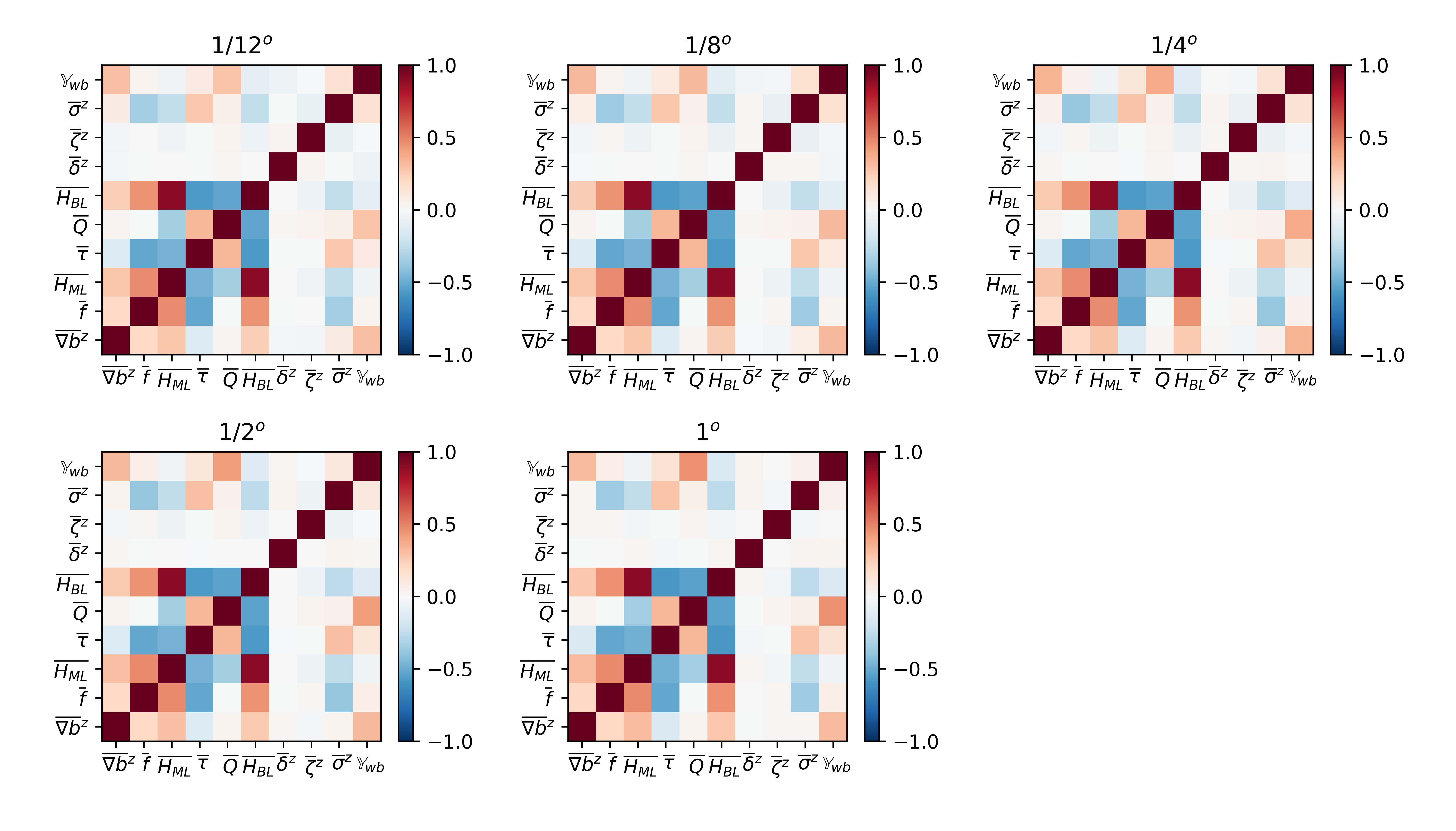
We choose to include input features that are correlated (Fig. S4), or have known analytical relationships, with submesoscale VBF. We leverage the physical relevance demonstrated by variables that appear in the MLE parameterization [Fox-Kemper \BOthers. (\APACyear2011), Bodner \BOthers. (\APACyear2023)], as well as correlated large-scale velocity derivatives [<]e.g.,¿[]barkan2019role, balwada2021vertical,zhang2023parameterizing. The input features (Tab. 1) consist of the depth-averaged horizontal buoyancy gradient magnitude, , where buoyancy is defined as , and m/s2 is the gravity acceleration; Coriolis parameter, ; mixed layer depth, ; surface heat flux ,; surface wind stress magnitude, ; boundary layer depth, , an output of the LLC4320 computed from the Richardson number criteria with the critical value of 0.3 [<] K‐profile Parameterization,¿[]large1994oceanic; depth-averaged strain magnitude, ; depth-averaged vertical vorticity, ; depth-averaged horizontal divergence, . Note that velocities and wind stresses are all interpolated to collocate with the tracer grid.
Formally, we define our 9 input features as,
| (3) |
and a single output as,
| (4) |
The CNN provides a prediction of the subgrid fluxes as a function of the large scale variables, such that and , where represents the CNN and its prediction. Fig. 3 illustrates a schematic of the CNN with 9 input features and one output.
| CNN inputs, | |
|---|---|
| Depth-averaged buoyancy gradient magnitude | |
| Coriolis parameter | |
| Mixed layer depth | |
| Surface heat flux | |
| Surface wind stress magnitude | |
| Boundary layer depth | |
| Depth-averaged strain magnitude | |
| Depth-averaged vertical vorticity | |
| Depth-averaged horizontal divergence | |
| CNN Output, | |
| Depth-averaged subgrid vertical buoyancy flux |

2.3 CNN architecture and training
Each experiment, designed with a given filter scale, is trained and tested independently, but all CNNs shared a common architecture. We use a CNN architecture for regression inspired by applications for mesoscale eddy parameterizations [Bolton \BBA Zanna (\APACyear2019), Guillaumin \BBA Zanna (\APACyear2021), Perezhogin \BOthers. (\APACyear2023)]. A hyper-parameter sweep over the number of hidden layers, kernel size, learning rate, and weight decay, was used to find the best performing CNN. The CNN is trained over 100 epochs while minimizing the Mean Squared Error (MSE) loss (shown in Fig. S1). The hyperparameters were tuned against the filter scale experiment, and remained fixed throughout all other experiments. Results presented here are based on a CNN with a kernel size of 5X5 in the first layer, followed by 7 hidden convolutional layers with kernel size of 3x3, a learning rate of , and weight decay of . The total number of learnable parameters is approximately .
Prior to applying the CNN, all variables listed in Tab. 1 are normalized by a single mean and standard deviation computed over all regions (example shown in Fig. S2). To train the CNN, we randomly select 80% of the samples given from all regions combined. The remaining 20% is left unseen by the CNN, and is used to test the CNN prediction. Results are compared in the following section with the target LLC4320 data and the \citeAbodner2023modifying version of the MLE parameterization, which is used here as a baseline. In subsections 3.1 and 3.2, we examine other split choices between the train and test datasets to include subsets of the sampled regions or timeseries, respectively.
3 CNN prediction of subgrid submesoscale fluxes
Once trained, the CNN has learned a functional mapping, , between the input features, , and subgrid mixed layer VBF, . In this section, we examine the extent to which the CNN can make skillful predictions on data that was not included in the training process. For this purpose, we compare the CNN prediction with the target LLC4320 data held out from training, and test whether the CNN improves on the baseline given by the \citeAbodner2023modifying version of the MLE parameterization.
Illustrated by an example from the filter scale experiment (Fig. 4), the CNN is able to capture much of the fine-scale structure and sign of the subgrid VBF. The majority of the fluxes are positive, which is the bulk restratification effect inferred by the MLE parameterization. The negative fluxes exhibited in the LLC4320, and captured by the CNN but not the MLE parameterization, may be indicative of frontogenesis, where an ageostrophic secondary circulation intensifies the front [<]e.g.,¿[]hoskins1972atmospheric,shakespeare2013generalized. This can be further seen in the joint histogram of the VBF given by the target LLC4320 and those predicted by the CNN and MLE parameterizations (Fig. 5). The joint histograms are computed over the entire unseen test dataset, which provides a comparison over several orders of magnitude of the VBF. In the case of positive fluxes, the CNN prediction remains close to the LLC4320 VBF, as can be seen by the alignment along the one-to-one gray line, an improvement on the MLE parameterization which deviates from the LLC4320 VBF. For the negative fluxes, the one-to-one alignment is less pronounced, likely due to the significantly smaller number of negative samples seen by the CNN (less than of the total samples). However, the ability of the CNN to predict of negative fluxes is still an improvement on the MLE parameterization, which does not include negative fluxes by construction.
To test whether the CNN also has skill in predicting bulk effects, such as is inferred by the MLE parameterization, the CNN predictions on unseen test data are averaged over each month to form a seasonal cycle, and is compared with the equivalent for the MLE parameterization and LLC4320 target data. We find that in all regions, the CNN prediction captures the seasonality and bulk effects of the LLC4320 data, and outperforms the MLE parameterization, particularly where fluxes appear to be strongest during the winter and spring months where the LLC4320 VBF can be as large as three times the MLE prediction (Fig. 6 for the filter scale experiment and more quantitatively in the analysis described below).
Prediction skill of the CNN and MLE parameterization for all filter scales are quantified in terms of values relative to the LLC4320 target data (calculation described in more detail in Eq. (S1)). We find that the CNN remain at a value of at least 0.2 higher than that of the MLE in all filter scale experiments and in all regions (Fig. 7). As the magnitude of varies spatially (Fig. 2), this impacts the predicted output of the CNN in the different regions. The largest filter scales tend to have skill nearing an values of 1, which then decreases as the filter scale becomes smaller. In the large filter scale experiments, the fields tend to be smoother, as much of the subgrid spatial variability is averaged out, thus presenting an easier learning problem for the CNN. The CNN prediction skill is found to be especially sensitive in the small filter scale experiments, where it performs well in some regions, e.g. in the California Current where all values are above 0.8, but less so in others, e.g. in the Indian Ocean region where the values in the small filter scale experiments are below 0.3). In the regions that exhibit large sensitivity to the filter scale such as the Kuroshio Current, Indian Ocean, and South Pacific, the skill of the MLE parameterization drops significantly as well.
It is worth noting that the CNN prediction skill can be sensitive to the initialization weights even when training identical experiment configurations [<]e.g.,¿[]otness2023data. However, we find that for each given filter scale experiment, the sensitivity to the initialization weights is smaller than an value of 0.1 (Fig. S5), indicating that the large range of values displayed in Fig. 9 reflects the sensitivity due to regional variability rather than properties of the CNN.


As submesoscale seasonality greatly impacts the variability of VBF (demonstrated in Fig. 6), we examine the skill (in terms of values) of the CNN and MLE parameterization averaged only over winter and summer months (Fig. 8). During winter, when mixed layer VBF tend to be stronger, the skill of both the CNN and MLE parameterization in the smaller filter scale experiments drops compared with its equivalent in summer. This is particularly true for regions where fluxes are very strong during winter, such as in the Kuroshio Current, where the and filter scale experiments shows no skill (negative ) during winter compared with an value above in summer. Similarly, the Gulf Stream, Agulhas Current, Malvinas Current, and the Southern Ocean near New Zealand all exhibit a drop in skill in both the MLE and CNN with small filter scales. In other regions with less of a pronounced seasonal cycle, such as in the South Pacific or South Atlantic regions, where the CNN skill is roughly the same for summer and winter, and differences appear within the range that can be explained by the CNN initialization sensitivity. Interestingly, the values of the MLE parameterization still drops in both regions during winter in all filter scale experiments. These results suggest that both the CNN and the MLE parameterization struggle to predict the strongest fluxes, generally exhibited during winter and spring months [<]e.g.,¿[]callies2015seasonality,johnson2016global.
To better understand the dependency of our method on the training data, and in particular on regional and seasonal variability, in the following subsections we perform two sensitivity tests by holding out parts of the training data, retraining the CNN, and examining CNN prediction skill on unseen regions or selected fractions of the timeseries.
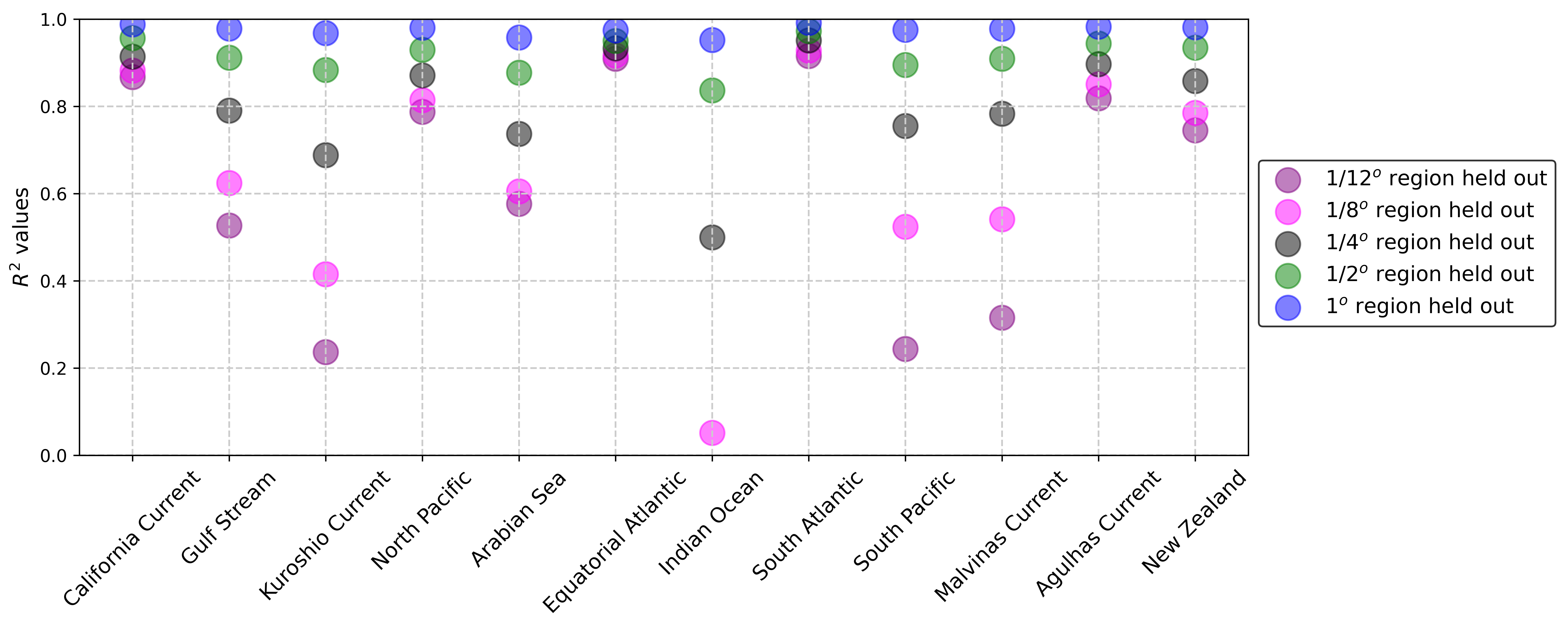
3.1 Holding out regions from training
We test the ability of the CNN to make predictions on regions that are not included in the training data. We thus generate 12 new datasets that correspond to removing one region at a time from the training dataset. We retrain the CNN in 12 different experiments, and make predictions on a different unseen region each time. The values of the CNN on the unseen regional data (Fig. 9) remain consistent with those found on the full training set (Fig. 7) across filter scales and over all regions. This suggests that the training data covers a wide enough range of dynamical regimes that enables generalization of the CNN on regions not included in training, an especially important result given that a fairly small number of regions were included in training compared with the full ocean.
3.2 Holding out seasonality from training
We perform two experiments in which we hold out winter and summer months from the training data, to examine the ability of the CNN to make predictions on unseen seasonal variability. We thus create two new training and test datasets to better understand the overall sensitivity of our method to submesoscale seasonality:
-
•
Winter held out refers to training data which excludes from the time series the months of January, February, March from all regions in the Northern Hemisphere, and July, August, September from regions in the Southern Hemisphere. Note again that we have removed equatorial regions from the analysis entirely. The remainder of the time series– e.g. spring, summer, fall– is used to train the CNN, and predictions are made on the unseen winter data.
-
•
Summer held out is same as the above, where we now exclude July, August, September from the Northern Hemisphere and January, February, March from the Southern Hemisphere. Equatorial regions are once again excluded.
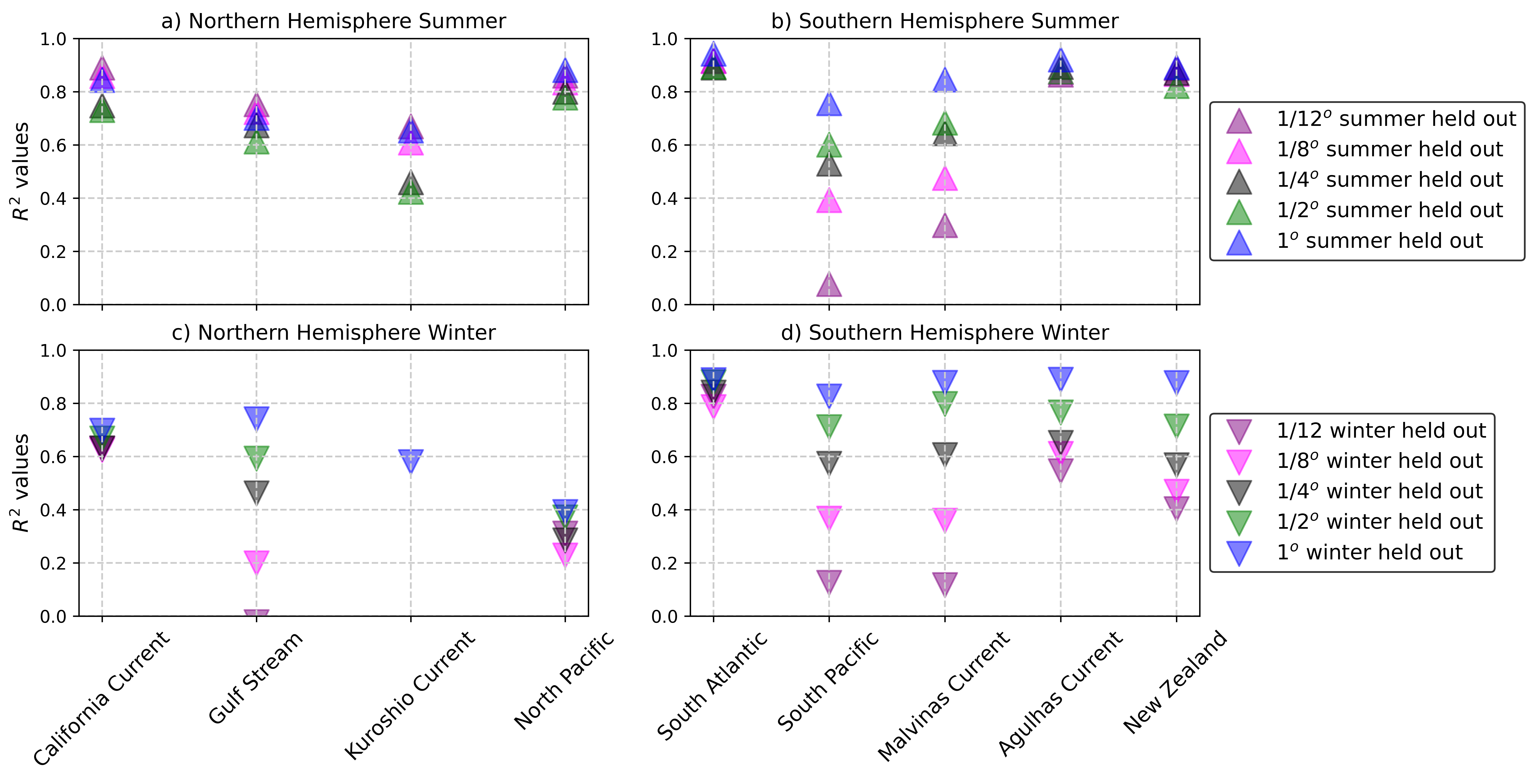
In these experiments, we find that results differ between regions in the Northern and Southern Hemispheres. In the Northern Hemisphere regions, the values in the ”Summer held out” experiments decrease by a margin larger than 0.1 compared with the CNN trained on the full timeseries (Fig. 10a compared with Fig. 8). We find the largest decreases in particular in the small filter scale experiments in regions affected by strong ocean boundary currents (i.e., the Gulf Stream and Kuroshio Current). Contrarily, the Southern Hemisphere regions are found to be consistent with the predictions for experiments trained on the full timeseries (Fig. 10b and Fig. 8). The CNN predictions in the ”Winter held out” experiments result in lower values in the Northern Hemisphere (Fig. 10c) compared with predictions trained on the the full timeseries. In the Kuroshio Current for example, all filter scales smaller than result in negative values, indicating that there is no skill in the CNN prediction in these cases. In the Southern Hemisphere regions (Fig. 10d), the ”Winter held out” experiments also display a decrease in values but it is still within the margin that can be explained by sensitivity to the initialization weights (Fig. S5). These results reinforce the need for the distribution of the data used to train the CNN to include the strongest seasonal fluxes, and particularly from regions where submesoscales are most active, such as near ocean boundary currents.
Results from both the seasonal and regional sensitivity experiments indicate that the learned relationships between the input features and can extend over a variety of dynamical regimes, especially in the large filter scale experiments. In the following section we delve deeper in attempt to interpret these relationships.
4 Local and non-local feature importance
We have shown that the CNN improves on the MLE parameterization, but an important remaining question is why? What relationships are learned between the input variables and that lead to better predictions by the CNN? With such complex and nonlinear relationships, it is difficult to decipher which input feature is most important and for what reason. Many methods exist that help explain and interpret the dependency of CNN outputs to its inputs [<]e.g.,¿[] zeiler2014visualizing, ribeiro2016should, selvaraju2017grad, van2022tractability. Here, we have chosen two complimentary methods that help gain insight on the learned relationships and the importance of individual inputs to .
4.1 Impact of input feature on CNN prediction skill
To test the dependency of the CNN prediction on certain input features, we perform a set of ablation experiments, where we remove one input feature at a time, retrain the CNN, and examine the resulting prediction skill in terms of the relative value. This relative value is taken as the difference between , resulting from the experiment with all input features included, and , resulting from the ablation experiment for each input. A high value indicates that the skill has dropped in a particular ablation experiment, meaning that the CNN strongly depends on said input feature (top panels in Fig. 11). Notably, strain demonstrates the strongest dependency of the CNN consistently across all filter scales. Interestingly, there appears to be very little sensitivity to the removal of any other input feature, including those used by the MLE parameterization.

4.2 Sensitivity of output relative to input features
We next apply a complimentary method to the ablation experiment above. The Jacobian of the CNN prediction, ), is computed with respect to the input features by taking gradients along the CNN weights, . The Jacobian is an especially useful metric to evaluate the point-wise sensitivity of the output to each input feature [<]e.g.,¿[]ross2023benchmarking. Note that unlike the ablation experiment, where we examined the value on the full output domain, the Jacobian considers only the sensitivity of a single output grid cell to a single grid cell in the input feature map. Here, we compute the Jacobian over the entire unseen test dataset, and examine its average values for each input feature, thus providing a metric for how sensitive, on average, the CNN output is to each input feature. We contrast the Jacobian with the values given by the ablation experiments (Fig. 11), where for the Jacobian, a high score indicates that the CNN prediction, , is sensitive to point-wise changes in a certain input. We find that the highest-ranked input feature, for which is most sensitive to, is the mixed layer depth, , which is generally a one-dimensional, local property determined by surface forcing. The sensitivity to mixed layer depth is followed by sensitivity to boundary layer depth, the buoyancy gradient, and vorticity. Note that does not appear to be sensitive to point-wise changes in surface heat flux, surface wind stress, or Coriolis, which is likely due to these fields being smoother in the LLC4320 at the scales relevant for the Jacobian. Despite strain being the most important feature in the previous section, it is only in the filter scale experiment that the Jacobian exhibits sensitivity of to vorticity, divergence, and strain, indicating that the impact of these fields is most apparent at the large scale.
4.3 Receptive field of the CNN
To further understand the relevance of locality, we follow the analysis in \citeAross2023benchmarking for examining the Jacobian of the output center point with respect to the full domain of each input feature. An example for the buoyancy gradient input feature is shown in Fig. 12a, where the shaded area illustrates the CNN’s receptive field needed to predict a single output point. Averaging over that halo, we examine the fraction of Jacobian over the number of grid points, which can be thought of as the percentage of sensitivity for each input feature that is being captured by the CNN (Fig. 12b,c). We find that 7 grid points away from the center is sufficient for capturing 90% of the Jacobian fraction, e.g. 90% of sensitivity between the output and input features. A relatively local receptive field is found to be consistent across filter scales despite the varying importance of input features found previously.
This result complements the analysis in \citeAgultekin2024analysis, which found that the \citeAguillaumin2021stochastic CNN skill saturates at a stencil of seven grid points for coarse-graining factors of 4, 8, 12, 16. As discussed in 2.3, the CNN architecture choice used here is motivated by that used in \citeAguillaumin2021stochastic, however, the physical phenomena we are parameterizing is different, and so are the input and output features. An investigation of the significance of a seven grid point stencil and its dependence on the CNN architecture in both cases is left for a future study.

5 Discussion and Conclusions
The parameterization for submesoscale VBF plays a key role in setting stratification in the ocean mixed layer, and as such contributes to the exchange between the ocean and atmosphere systems in GCMs. In contrast to previous physics-based approaches, here we develop a new data-driven parameterization, where a CNN is trained to predict mixed layer VBF. The subgrid flux, , is inferred by the CNN as a function of 9 large-scale input features with known relevance to submesoscale VBF: , , , , , , , , , (see Tab. 1). The data used for training is given from 12 regions sampled from the global high-resolution LLC4320 simulation output. The CNN is trained over a random selection of of all data, while the remaining is unseen by the CNN and is used for testing. We perform five filter scale experiments of and compare with a baseline given by the \citeAbodner2023modifying formulation of the MLE parameterization.
We consistently find that the CNN predictions improve on the MLE parameterization, with higher values across all regions, seasons, and filter scales tested in this study. We additionally perform several sensitivity experiments, where we test the CNN’s ability to make predictions on regional or temporal data held out during training. It is found that the CNN, in particular in the larger filter scale experiments, is able to make skillful predictions on unseen data, but does poorly during when submesoscales are most active, generally corresponding to winter months and near ocean boundary currents.
The significant improvement on the MLE parameterization indicates that the CNN has learned new meaningful relationships between the input features and , such that it is able to make skillful predictions over widely different dynamical regimes. We applied two complimentary explainability methods which enable a closer look at the relationships between the CNN output and input features. We find that the CNN exhibits strong dependency on the local relationship between and the mixed layer depth, a 1D property driven by surface forcing, and strong non-local dependency on the large scale strain field, a variable closely related to frontogenesis, which is currently missing from the MLE parameterization in GCMs.
An important limitation of these method is in detecting the importance of features that are strongly correlated with other fields, such that removing one feature may not lead to differences in the CNN prediction skill. In particular, fields associated with surface forcing, e.g., mixed layer, boundary layer, surface heat flux, and wind stress are expected to be correlated (as is also found to be true in the LLC4320 data, Fig. S4). Nonetheless, results from the ablation experiments suggest that the primary reason the CNN predictions surpass those of the MLE parameterization are due to the newly-captured non-local relationship between and the large scale strain field, on which the CNN is strongly dependent. Note that strain is known for its role in constraining submesoscale fluxes and contributing to frontal intensification [<]e.g.,¿[]shcherbina2013statistics, balwada2021vertical,sinha2023submesoscales, but these findings emphasize the relevance of strain to improving submesoscale VBF parameterizations, such as recently proposed by \citeAzhang2023parameterizing. An extension of these approaches may include incorporating more data from other submesoscale permitting simulations [Uchida \BOthers. (\APACyear2022), Gultekin \BOthers. (\APACyear2024)], or an investigation of causal links which are not captures in the current framework [<]e.g.,¿[]camps2023discovering. An equation discovery approach [<]e.g.,¿[]zanna2020data may enable a closer comparison with \citeAzhang2023parameterizing, and whether the relationship between strain and submesoscale fluxes emerge in a similar fashion.
We have demonstrated that the CNN improves on the MLE parameterization in an offline setting. However, it is important to note that during training, the CNN minimizes the MSE loss– a metric closely related to the value (as shown in Eq. (S1)). The MLE parameterization, on the other hand, is designed to represent the bulk effects of submesoscale VBF. A next important step is to explore the implications of better captured mixed layer VBF in a GCM and compare with the MLE parameterization online, such as in a recent attempt by \citeAzhou2024neural in Regional Ocean Modeling System (ROMS). We have designed our method to correspond with the existing implementation of the MLE parameterization in GCMs, where the theoretical expression for in Eq. (S2) can simply be replaced with the CNN. A relatively small receptive field of 7 grid points is found to be sufficient at capturing relationships between the input features and , which suggests that a smaller network may aid future implementation efforts in GCMs [C. Zhang \BOthers. (\APACyear2023)]. A decomposition may be preferred to distinguish the bulk restratification effect with the intermittent negative fluxes, and will allow a more natural relationship with vertical buoyancy fluxes already estimated in boundary layer turbulence parameterizations [Large \BOthers. (\APACyear1994), Reichl \BBA Hallberg (\APACyear2018), Sane \BOthers. (\APACyear2023)]. The exact formulation, implementation, and evaluation of impact on climate variables is left for future work.
Beyond the modeling framework discussed above, the utility of our work can also be made amenable to observational data. In particular, the Surface Water and Ocean Topography (SWOT) altimeter mission is starting to provide measurements of sea surface height at an unprecedented resolution [Morrow \BOthers. (\APACyear2019)]. The data-driven approach presented here provides an opportunity to leverage surface fields derived from SWOT [<]e.g.,¿[]qiu2016reconstructability,bolton2019applications, to infer subsurface VBF and gain new insights of upper ocean dynamics.
Open data
Data from the LLC4320 simulation can be accessed using the llcreader Python package [Abernathey (\APACyear2019)]. Variables from the LLC4320 output in the regions used in this study are stored on the LEAP-Catalog https://catalog.leap.columbia.edu/feedstock/highresolution-ocean-simulation-llc4320-12hourly-averaged-3d-regions. Code used to process the LLC4320, train the CNN, and generate the figures in this manuscript can be found at https://github.com/abodner/submeso_param_net. Diagnostics incorporate open source Python packages: xhistogram, xhistogram.readthedocs.io; fastjmd95, [Abernathey (\APACyear2020)] ; xmitgcm, [Abernathey \BOthers. (\APACyear2021)].
Acknowledgements
This research received support through Schmidt Sciences, LLC. AB was supported by a grant from the Simons Foundation: award number 855143, Bodner. We thank members of the M2LInES project for support and constructive feedback during the formulation of ideas, in particular, Pavel Perezhogin, Chris Pedersen, Ryan Abernathey, Carlos Fernandez-Granda, and Fabrizio Falasca. The authors would also like to thank the Pangeo Project for providing open-source code which enabled timely analysis for working with the LLC4320 data. This research was also supported in part through the NYU IT High Performance Computing resources, services, and staff expertise.
References
- Abernathey (\APACyear2019) \APACinsertmetastarabernathey2019petabytes{APACrefauthors}Abernathey, R. \APACrefYearMonthDay2019. \APACrefbtitlePetabytes of Ocean Data, Part I: NASA ECCO Data Portal. Petabytes of ocean data, part i: Nasa ecco data portal. \PrintBackRefs\CurrentBib
- Abernathey (\APACyear2020) \APACinsertmetastarabernathey2020fastjmd95{APACrefauthors}Abernathey, R. \APACrefYearMonthDay2020. \BBOQ\APACrefatitlefastjmd95: Numba implementation of Jackett & McDougall (1995) ocean equation of state fastjmd95: Numba implementation of jackett & mcdougall (1995) ocean equation of state.\BBCQ \APACjournalVolNumPagesZenodo [code]10. \PrintBackRefs\CurrentBib
- Abernathey \BOthers. (\APACyear2021) \APACinsertmetastarabernathey2021xgcm{APACrefauthors}Abernathey, R., Busecke, J., Smith, T., Banihirwe, A., Fernandes, F., Bourbeau, J.\BDBLothers \APACrefYearMonthDay2021. \BBOQ\APACrefatitlexgcm: General circulation model postprocessing with xarray xgcm: General circulation model postprocessing with xarray.\BBCQ \APACjournalVolNumPagesZenodo [code]10. \PrintBackRefs\CurrentBib
- Ajayi \BOthers. (\APACyear2021) \APACinsertmetastarajayi2021diagnosing{APACrefauthors}Ajayi, A., Le Sommer, J., Chassignet, E\BPBIP., Molines, J\BHBIM., Xu, X., Albert, A.\BCBL \BBA Dewar, W. \APACrefYearMonthDay2021. \BBOQ\APACrefatitleDiagnosing cross-scale kinetic energy exchanges from two submesoscale permitting ocean models Diagnosing cross-scale kinetic energy exchanges from two submesoscale permitting ocean models.\BBCQ \APACjournalVolNumPagesJournal of Advances in Modeling Earth Systems136e2019MS001923. \PrintBackRefs\CurrentBib
- Bachman \BOthers. (\APACyear2017) \APACinsertmetastarbachman2017parameterization{APACrefauthors}Bachman, S\BPBID., Fox-Kemper, B., Taylor, J\BPBIR.\BCBL \BBA Thomas, L\BPBIN. \APACrefYearMonthDay2017. \BBOQ\APACrefatitleParameterization of frontal symmetric instabilities. I: Theory for resolved fronts Parameterization of frontal symmetric instabilities. i: Theory for resolved fronts.\BBCQ \APACjournalVolNumPagesOcean Modelling10972–95. \PrintBackRefs\CurrentBib
- Balwada \BOthers. (\APACyear2018) \APACinsertmetastarbalwada2018submesoscale{APACrefauthors}Balwada, D., Smith, K\BPBIS.\BCBL \BBA Abernathey, R. \APACrefYearMonthDay2018. \BBOQ\APACrefatitleSubmesoscale vertical velocities enhance tracer subduction in an idealized Antarctic Circumpolar Current Submesoscale vertical velocities enhance tracer subduction in an idealized antarctic circumpolar current.\BBCQ \APACjournalVolNumPagesGeophysical Research Letters45189790–9802. \PrintBackRefs\CurrentBib
- Balwada \BOthers. (\APACyear2021) \APACinsertmetastarbalwada2021vertical{APACrefauthors}Balwada, D., Xiao, Q., Smith, S., Abernathey, R.\BCBL \BBA Gray, A\BPBIR. \APACrefYearMonthDay2021. \BBOQ\APACrefatitleVertical fluxes conditioned on vorticity and strain reveal submesoscale ventilation Vertical fluxes conditioned on vorticity and strain reveal submesoscale ventilation.\BBCQ \APACjournalVolNumPagesJournal of Physical Oceanography5192883–2901. \PrintBackRefs\CurrentBib
- Barkan \BOthers. (\APACyear2019) \APACinsertmetastarbarkan2019role{APACrefauthors}Barkan, R., Molemaker, M\BPBIJ., Srinivasan, K., McWilliams, J\BPBIC.\BCBL \BBA D’Asaro, E\BPBIA. \APACrefYearMonthDay2019. \BBOQ\APACrefatitleThe role of horizontal divergence in submesoscale frontogenesis The role of horizontal divergence in submesoscale frontogenesis.\BBCQ \APACjournalVolNumPagesJournal of Physical Oceanography4961593–1618. \PrintBackRefs\CurrentBib
- Boccaletti \BOthers. (\APACyear2007) \APACinsertmetastarboccaletti2007mixed{APACrefauthors}Boccaletti, G., Ferrari, R.\BCBL \BBA Fox-Kemper, B. \APACrefYearMonthDay2007. \BBOQ\APACrefatitleMixed layer instabilities and restratification Mixed layer instabilities and restratification.\BBCQ \APACjournalVolNumPagesJournal of Physical Oceanography3792228–2250. \PrintBackRefs\CurrentBib
- Bodner \BOthers. (\APACyear2023) \APACinsertmetastarbodner2023modifying{APACrefauthors}Bodner, A\BPBIS., Fox-Kemper, B., Johnson, L., Van Roekel, L\BPBIP., McWilliams, J\BPBIC., Sullivan, P\BPBIP.\BDBLDong, J. \APACrefYearMonthDay2023. \BBOQ\APACrefatitleModifying the Mixed Layer Eddy Parameterization to Include Frontogenesis Arrest by Boundary Layer Turbulence Modifying the mixed layer eddy parameterization to include frontogenesis arrest by boundary layer turbulence.\BBCQ \APACjournalVolNumPagesJournal of Physical Oceanography531323–339. \PrintBackRefs\CurrentBib
- Bolton \BBA Zanna (\APACyear2019) \APACinsertmetastarbolton2019applications{APACrefauthors}Bolton, T.\BCBT \BBA Zanna, L. \APACrefYearMonthDay2019. \BBOQ\APACrefatitleApplications of deep learning to ocean data inference and subgrid parameterization Applications of deep learning to ocean data inference and subgrid parameterization.\BBCQ \APACjournalVolNumPagesJournal of Advances in Modeling Earth Systems111376–399. \PrintBackRefs\CurrentBib
- Bopp \BOthers. (\APACyear2015) \APACinsertmetastarbopp2015pathways{APACrefauthors}Bopp, L., Lévy, M., Resplandy, L.\BCBL \BBA Sallée, J\BHBIB. \APACrefYearMonthDay2015. \BBOQ\APACrefatitlePathways of anthropogenic carbon subduction in the global ocean Pathways of anthropogenic carbon subduction in the global ocean.\BBCQ \APACjournalVolNumPagesGeophysical Research Letters42156416–6423. \PrintBackRefs\CurrentBib
- Callies \BBA Ferrari (\APACyear2018) \APACinsertmetastarcallies2018baroclinic{APACrefauthors}Callies, J.\BCBT \BBA Ferrari, R. \APACrefYearMonthDay2018. \BBOQ\APACrefatitleBaroclinic instability in the presence of convection Baroclinic instability in the presence of convection.\BBCQ \APACjournalVolNumPagesJournal of Physical Oceanography48145–60. \PrintBackRefs\CurrentBib
- Callies \BOthers. (\APACyear2015) \APACinsertmetastarcallies2015seasonality{APACrefauthors}Callies, J., Ferrari, R., Klymak, J\BPBIM.\BCBL \BBA Gula, J. \APACrefYearMonthDay2015. \BBOQ\APACrefatitleSeasonality in submesoscale turbulence Seasonality in submesoscale turbulence.\BBCQ \APACjournalVolNumPagesNature communications616862. \PrintBackRefs\CurrentBib
- Camps-Valls \BOthers. (\APACyear2023) \APACinsertmetastarcamps2023discovering{APACrefauthors}Camps-Valls, G., Gerhardus, A., Ninad, U., Varando, G., Martius, G., Balaguer-Ballester, E.\BDBLRunge, J. \APACrefYearMonthDay2023. \BBOQ\APACrefatitleDiscovering causal relations and equations from data Discovering causal relations and equations from data.\BBCQ \APACjournalVolNumPagesPhysics Reports10441–68. \PrintBackRefs\CurrentBib
- Chattopadhyay \BOthers. (\APACyear2020) \APACinsertmetastarchattopadhyay2020predicting{APACrefauthors}Chattopadhyay, A., Hassanzadeh, P.\BCBL \BBA Pasha, S. \APACrefYearMonthDay2020. \BBOQ\APACrefatitlePredicting clustered weather patterns: A test case for applications of convolutional neural networks to spatio-temporal climate data Predicting clustered weather patterns: A test case for applications of convolutional neural networks to spatio-temporal climate data.\BBCQ \APACjournalVolNumPagesScientific reports1011317. \PrintBackRefs\CurrentBib
- Dagon \BOthers. (\APACyear2022) \APACinsertmetastardagon2022machine{APACrefauthors}Dagon, K., Truesdale, J., Biard, J\BPBIC., Kunkel, K\BPBIE., Meehl, G\BPBIA.\BCBL \BBA Molina, M\BPBIJ. \APACrefYearMonthDay2022. \BBOQ\APACrefatitleMachine Learning-Based Detection of Weather Fronts and Associated Extreme Precipitation in Historical and Future Climates Machine learning-based detection of weather fronts and associated extreme precipitation in historical and future climates.\BBCQ \APACjournalVolNumPagesJournal of Geophysical Research: Atmospheres12721e2022JD037038. \PrintBackRefs\CurrentBib
- de Boyer Montégut \BOthers. (\APACyear2004) \APACinsertmetastarde2004mixed{APACrefauthors}de Boyer Montégut, C., Madec, G., Fischer, A\BPBIS., Lazar, A.\BCBL \BBA Iudicone, D. \APACrefYearMonthDay2004. \BBOQ\APACrefatitleMixed layer depth over the global ocean: An examination of profile data and a profile-based climatology Mixed layer depth over the global ocean: An examination of profile data and a profile-based climatology.\BBCQ \APACjournalVolNumPagesJournal of Geophysical Research: Oceans109C12. \PrintBackRefs\CurrentBib
- Forget \BOthers. (\APACyear2015) \APACinsertmetastarforget2015ecco{APACrefauthors}Forget, G., Campin, J\BHBIM., Heimbach, P., Hill, C., Ponte, R.\BCBL \BBA Wunsch, C. \APACrefYearMonthDay2015. \BBOQ\APACrefatitleECCO version 4: An integrated framework for non-linear inverse modeling and global ocean state estimation Ecco version 4: An integrated framework for non-linear inverse modeling and global ocean state estimation.\BBCQ \APACjournalVolNumPagesGeoscientific Model Development8103071–3104. \PrintBackRefs\CurrentBib
- Fox-Kemper \BOthers. (\APACyear2011) \APACinsertmetastarfox2011parameterization{APACrefauthors}Fox-Kemper, B., Danabasoglu, G., Ferrari, R., Griffies, S., Hallberg, R., Holland, M.\BDBLSamuels, B. \APACrefYearMonthDay2011. \BBOQ\APACrefatitleParameterization of mixed layer eddies. III: Implementation and impact in global ocean climate simulations Parameterization of mixed layer eddies. iii: Implementation and impact in global ocean climate simulations.\BBCQ \APACjournalVolNumPagesOcean Modelling391-261–78. \PrintBackRefs\CurrentBib
- Fox-Kemper \BOthers. (\APACyear2008) \APACinsertmetastarfox2008parameterization{APACrefauthors}Fox-Kemper, B., Ferrari, R.\BCBL \BBA Hallberg, R. \APACrefYearMonthDay2008. \BBOQ\APACrefatitleParameterization of mixed layer eddies. Part I: Theory and diagnosis Parameterization of mixed layer eddies. part i: Theory and diagnosis.\BBCQ \APACjournalVolNumPagesJournal of Physical Oceanography3861145–1165. \PrintBackRefs\CurrentBib
- Frankignoul \BBA Hasselmann (\APACyear1977) \APACinsertmetastarfrankignoul1977stochastic{APACrefauthors}Frankignoul, C.\BCBT \BBA Hasselmann, K. \APACrefYearMonthDay1977. \BBOQ\APACrefatitleStochastic climate models, Part II Application to sea-surface temperature anomalies and thermocline variability Stochastic climate models, part ii application to sea-surface temperature anomalies and thermocline variability.\BBCQ \APACjournalVolNumPagesTellus294289–305. \PrintBackRefs\CurrentBib
- Gallmeier \BOthers. (\APACyear2023) \APACinsertmetastargallmeier2023evaluation{APACrefauthors}Gallmeier, K\BPBIM., Prochaska, J\BPBIX., Cornillon, P., Menemenlis, D.\BCBL \BBA Kelm, M. \APACrefYearMonthDay2023. \BBOQ\APACrefatitleAn evaluation of the LLC4320 global ocean simulation based on the submesoscale structure of modeled sea surface temperature fields An evaluation of the llc4320 global ocean simulation based on the submesoscale structure of modeled sea surface temperature fields.\BBCQ \APACjournalVolNumPagesGeoscientific Model Development Discussions1–42. \PrintBackRefs\CurrentBib
- Guillaumin \BBA Zanna (\APACyear2021) \APACinsertmetastarguillaumin2021stochastic{APACrefauthors}Guillaumin, A\BPBIP.\BCBT \BBA Zanna, L. \APACrefYearMonthDay2021. \BBOQ\APACrefatitleStochastic-deep learning parameterization of ocean momentum forcing Stochastic-deep learning parameterization of ocean momentum forcing.\BBCQ \APACjournalVolNumPagesJournal of Advances in Modeling Earth Systems139e2021MS002534. \PrintBackRefs\CurrentBib
- Gula \BOthers. (\APACyear2022) \APACinsertmetastargula2022submesoscale{APACrefauthors}Gula, J., Taylor, J., Shcherbina, A.\BCBL \BBA Mahadevan, A. \APACrefYearMonthDay2022. \BBOQ\APACrefatitleSubmesoscale processes and mixing Submesoscale processes and mixing.\BBCQ \BIn \APACrefbtitleOcean Mixing Ocean mixing (\BPGS 181–214). \APACaddressPublisherElsevier. \PrintBackRefs\CurrentBib
- Gultekin \BOthers. (\APACyear2024) \APACinsertmetastargultekin2024analysis{APACrefauthors}Gultekin, C., Subel, A., Zhang, C., Leibovich, M., Perezhogin, P., Adcroft, A.\BDBLZanna, L. \APACrefYearMonthDay2024. \BBOQ\APACrefatitleAn Analysis of Deep Learning Parameterizations for Ocean Subgrid Eddy Forcing An analysis of deep learning parameterizations for ocean subgrid eddy forcing.\BBCQ \APACjournalVolNumPagesarXiv preprint arXiv:2411.06604. \PrintBackRefs\CurrentBib
- Hoskins \BBA Bretherton (\APACyear1972) \APACinsertmetastarhoskins1972atmospheric{APACrefauthors}Hoskins, B\BPBIJ.\BCBT \BBA Bretherton, F\BPBIP. \APACrefYearMonthDay1972. \BBOQ\APACrefatitleAtmospheric frontogenesis models: Mathematical formulation and solution Atmospheric frontogenesis models: Mathematical formulation and solution.\BBCQ \APACjournalVolNumPagesJournal of the atmospheric sciences29111–37. \PrintBackRefs\CurrentBib
- IPCC (\APACyear2019) \APACinsertmetastarSROCC{APACrefauthors}IPCC. \APACrefYear2019. \APACrefbtitleSpecial Report on the Ocean and Cryosphere in a Changing Climate Special report on the ocean and cryosphere in a changing climate [Book]. \APACaddressPublisherCambridge, United Kingdom and New York, NY, USACambridge University Press. {APACrefDOI} 10.1017/9781009157964 \PrintBackRefs\CurrentBib
- IPCC (\APACyear2021) \APACinsertmetastarRN1{APACrefauthors}IPCC. \APACrefYear2021. \APACrefbtitleClimate Change 2021: The Physical Science Basis. Contribution of Working Group I to the Sixth Assessment Report of the Intergovernmental Panel on Climate Change Climate change 2021: The physical science basis. contribution of working group i to the sixth assessment report of the intergovernmental panel on climate change (\BVOL In Press) [Book]. \APACaddressPublisherCambridge, United Kingdom and New York, NY, USACambridge University Press. {APACrefDOI} 10.1017/9781009157896 \PrintBackRefs\CurrentBib
- Johnson \BOthers. (\APACyear2016) \APACinsertmetastarjohnson2016global{APACrefauthors}Johnson, L., Lee, C\BPBIM.\BCBL \BBA D’Asaro, E\BPBIA. \APACrefYearMonthDay2016. \BBOQ\APACrefatitleGlobal estimates of lateral springtime restratification Global estimates of lateral springtime restratification.\BBCQ \APACjournalVolNumPagesJournal of Physical Oceanography4651555–1573. \PrintBackRefs\CurrentBib
- Lapeyre \BOthers. (\APACyear2006) \APACinsertmetastarlapeyre2006oceanic{APACrefauthors}Lapeyre, G., Klein, P.\BCBL \BBA Hua, B\BPBIL. \APACrefYearMonthDay2006. \BBOQ\APACrefatitleOceanic restratification forced by surface frontogenesis Oceanic restratification forced by surface frontogenesis.\BBCQ \APACjournalVolNumPagesJournal of Physical Oceanography3681577–1590. \PrintBackRefs\CurrentBib
- Large \BOthers. (\APACyear1994) \APACinsertmetastarlarge1994oceanic{APACrefauthors}Large, W\BPBIG., McWilliams, J\BPBIC.\BCBL \BBA Doney, S\BPBIC. \APACrefYearMonthDay1994. \BBOQ\APACrefatitleOceanic vertical mixing: A review and a model with a nonlocal boundary layer parameterization Oceanic vertical mixing: A review and a model with a nonlocal boundary layer parameterization.\BBCQ \APACjournalVolNumPagesReviews of geophysics324363–403. \PrintBackRefs\CurrentBib
- Mahadevan \BOthers. (\APACyear2010) \APACinsertmetastarmahadevan2010rapid{APACrefauthors}Mahadevan, A., Tandon, A.\BCBL \BBA Ferrari, R. \APACrefYearMonthDay2010. \BBOQ\APACrefatitleRapid changes in mixed layer stratification driven by submesoscale instabilities and winds Rapid changes in mixed layer stratification driven by submesoscale instabilities and winds.\BBCQ \APACjournalVolNumPagesJournal of Geophysical Research: Oceans115C3. \PrintBackRefs\CurrentBib
- McWilliams (\APACyear2016) \APACinsertmetastarmcwilliams2016submesoscale{APACrefauthors}McWilliams, J\BPBIC. \APACrefYearMonthDay2016. \BBOQ\APACrefatitleSubmesoscale currents in the ocean Submesoscale currents in the ocean.\BBCQ \APACjournalVolNumPagesProceedings of the Royal Society A: Mathematical, Physical and Engineering Sciences472218920160117. \PrintBackRefs\CurrentBib
- Menemenlis \BOthers. (\APACyear2008) \APACinsertmetastarmenemenlis2008ecco2{APACrefauthors}Menemenlis, D., Campin, J\BHBIM., Heimbach, P., Hill, C., Lee, T., Nguyen, A.\BDBLZhang, H. \APACrefYearMonthDay2008. \BBOQ\APACrefatitleECCO2: High resolution global ocean and sea ice data synthesis Ecco2: High resolution global ocean and sea ice data synthesis.\BBCQ \APACjournalVolNumPagesMercator Ocean Quarterly Newsletter31October13–21. \PrintBackRefs\CurrentBib
- Menemenlis \BOthers. (\APACyear2021) \APACinsertmetastarmenemenlis2021pre{APACrefauthors}Menemenlis, D., Hill, C., Henze, C., Wang, J.\BCBL \BBA Fenty, I. \APACrefYearMonthDay2021. \APACrefbtitlePre-SWOT Level-4 Hourly MITgcm LLC4320 Native 2km Grid Oceanographic Version 1.0. Pre-swot level-4 hourly mitgcm llc4320 native 2km grid oceanographic version 1.0. \APACaddressPublisherVer. \PrintBackRefs\CurrentBib
- Morrow \BOthers. (\APACyear2019) \APACinsertmetastarmorrow2019global{APACrefauthors}Morrow, R., Fu, L\BHBIL., Ardhuin, F., Benkiran, M., Chapron, B., Cosme, E.\BDBLothers \APACrefYearMonthDay2019. \BBOQ\APACrefatitleGlobal observations of fine-scale ocean surface topography with the surface water and ocean topography (SWOT) mission Global observations of fine-scale ocean surface topography with the surface water and ocean topography (swot) mission.\BBCQ \APACjournalVolNumPagesFrontiers in Marine Science6232. \PrintBackRefs\CurrentBib
- Otness \BOthers. (\APACyear2023) \APACinsertmetastarotness2023data{APACrefauthors}Otness, K., Zanna, L.\BCBL \BBA Bruna, J. \APACrefYearMonthDay2023. \BBOQ\APACrefatitleData-driven multiscale modeling of subgrid parameterizations in climate models Data-driven multiscale modeling of subgrid parameterizations in climate models.\BBCQ \APACjournalVolNumPagesarXiv preprint arXiv:2303.17496. \PrintBackRefs\CurrentBib
- Perezhogin \BOthers. (\APACyear2023) \APACinsertmetastarperezhogin2023generative{APACrefauthors}Perezhogin, P., Zanna, L.\BCBL \BBA Fernandez-Granda, C. \APACrefYearMonthDay2023. \BBOQ\APACrefatitleGenerative data-driven approaches for stochastic subgrid parameterizations in an idealized ocean model Generative data-driven approaches for stochastic subgrid parameterizations in an idealized ocean model.\BBCQ \APACjournalVolNumPagesarXiv preprint arXiv:2302.07984. \PrintBackRefs\CurrentBib
- Qiu \BOthers. (\APACyear2016) \APACinsertmetastarqiu2016reconstructability{APACrefauthors}Qiu, B., Chen, S., Klein, P., Ubelmann, C., Fu, L\BHBIL.\BCBL \BBA Sasaki, H. \APACrefYearMonthDay2016. \BBOQ\APACrefatitleReconstructability of three-dimensional upper-ocean circulation from SWOT sea surface height measurements Reconstructability of three-dimensional upper-ocean circulation from swot sea surface height measurements.\BBCQ \APACjournalVolNumPagesJournal of Physical Oceanography463947–963. \PrintBackRefs\CurrentBib
- Reichl \BBA Hallberg (\APACyear2018) \APACinsertmetastarreichl2018simplified{APACrefauthors}Reichl, B\BPBIG.\BCBT \BBA Hallberg, R. \APACrefYearMonthDay2018. \BBOQ\APACrefatitleA simplified energetics based planetary boundary layer (ePBL) approach for ocean climate simulations. A simplified energetics based planetary boundary layer (epbl) approach for ocean climate simulations.\BBCQ \APACjournalVolNumPagesOcean Modelling132112–129. \PrintBackRefs\CurrentBib
- Ribeiro \BOthers. (\APACyear2016) \APACinsertmetastarribeiro2016should{APACrefauthors}Ribeiro, M\BPBIT., Singh, S.\BCBL \BBA Guestrin, C. \APACrefYearMonthDay2016. \BBOQ\APACrefatitle” Why should i trust you?” Explaining the predictions of any classifier ” why should i trust you?” explaining the predictions of any classifier.\BBCQ \BIn \APACrefbtitleProceedings of the 22nd ACM SIGKDD international conference on knowledge discovery and data mining Proceedings of the 22nd acm sigkdd international conference on knowledge discovery and data mining (\BPGS 1135–1144). \PrintBackRefs\CurrentBib
- Rocha \BOthers. (\APACyear2016) \APACinsertmetastarrocha2016mesoscale{APACrefauthors}Rocha, C\BPBIB., Chereskin, T\BPBIK., Gille, S\BPBIT.\BCBL \BBA Menemenlis, D. \APACrefYearMonthDay2016. \BBOQ\APACrefatitleMesoscale to submesoscale wavenumber spectra in Drake Passage Mesoscale to submesoscale wavenumber spectra in drake passage.\BBCQ \APACjournalVolNumPagesJournal of Physical Oceanography462601–620. \PrintBackRefs\CurrentBib
- Ross \BOthers. (\APACyear2023) \APACinsertmetastarross2023benchmarking{APACrefauthors}Ross, A., Li, Z., Perezhogin, P., Fernandez-Granda, C.\BCBL \BBA Zanna, L. \APACrefYearMonthDay2023. \BBOQ\APACrefatitleBenchmarking of machine learning ocean subgrid parameterizations in an idealized model Benchmarking of machine learning ocean subgrid parameterizations in an idealized model.\BBCQ \APACjournalVolNumPagesJournal of Advances in Modeling Earth Systems151e2022MS003258. \PrintBackRefs\CurrentBib
- Sagaut (\APACyear2005) \APACinsertmetastarsagaut2005large{APACrefauthors}Sagaut, P. \APACrefYear2005. \APACrefbtitleLarge eddy simulation for incompressible flows: an introduction Large eddy simulation for incompressible flows: an introduction. \APACaddressPublisherSpringer Science & Business Media. \PrintBackRefs\CurrentBib
- Sane \BOthers. (\APACyear2023) \APACinsertmetastarsane2023parameterizing{APACrefauthors}Sane, A., Reichl, B\BPBIG., Adcroft, A.\BCBL \BBA Zanna, L. \APACrefYearMonthDay2023. \BBOQ\APACrefatitleParameterizing Vertical Mixing Coefficients in the Ocean Surface Boundary Layer using Neural Networks Parameterizing vertical mixing coefficients in the ocean surface boundary layer using neural networks.\BBCQ \APACjournalVolNumPagesarXiv preprint arXiv:2306.09045. \PrintBackRefs\CurrentBib
- Selvaraju \BOthers. (\APACyear2017) \APACinsertmetastarselvaraju2017grad{APACrefauthors}Selvaraju, R\BPBIR., Cogswell, M., Das, A., Vedantam, R., Parikh, D.\BCBL \BBA Batra, D. \APACrefYearMonthDay2017. \BBOQ\APACrefatitleGrad-cam: Visual explanations from deep networks via gradient-based localization Grad-cam: Visual explanations from deep networks via gradient-based localization.\BBCQ \BIn \APACrefbtitleProceedings of the IEEE international conference on computer vision Proceedings of the ieee international conference on computer vision (\BPGS 618–626). \PrintBackRefs\CurrentBib
- Shakespeare \BBA Taylor (\APACyear2013) \APACinsertmetastarshakespeare2013generalized{APACrefauthors}Shakespeare, C\BPBIJ.\BCBT \BBA Taylor, J\BPBIR. \APACrefYearMonthDay2013. \BBOQ\APACrefatitleA generalized mathematical model of geostrophic adjustment and frontogenesis: uniform potential vorticity A generalized mathematical model of geostrophic adjustment and frontogenesis: uniform potential vorticity.\BBCQ \APACjournalVolNumPagesJournal of fluid mechanics736366–413. \PrintBackRefs\CurrentBib
- Shamekh \BOthers. (\APACyear2023) \APACinsertmetastarshamekh2023implicit{APACrefauthors}Shamekh, S., Lamb, K\BPBID., Huang, Y.\BCBL \BBA Gentine, P. \APACrefYearMonthDay2023. \BBOQ\APACrefatitleImplicit learning of convective organization explains precipitation stochasticity Implicit learning of convective organization explains precipitation stochasticity.\BBCQ \APACjournalVolNumPagesProceedings of the National Academy of Sciences12020e2216158120. \PrintBackRefs\CurrentBib
- Shcherbina \BOthers. (\APACyear2013) \APACinsertmetastarshcherbina2013statistics{APACrefauthors}Shcherbina, A\BPBIY., D’Asaro, E\BPBIA., Lee, C\BPBIM., Klymak, J\BPBIM., Molemaker, M\BPBIJ.\BCBL \BBA McWilliams, J\BPBIC. \APACrefYearMonthDay2013. \BBOQ\APACrefatitleStatistics of vertical vorticity, divergence, and strain in a developed submesoscale turbulence field Statistics of vertical vorticity, divergence, and strain in a developed submesoscale turbulence field.\BBCQ \APACjournalVolNumPagesGeophysical Research Letters40174706–4711. \PrintBackRefs\CurrentBib
- Sinha \BOthers. (\APACyear2023) \APACinsertmetastarsinha2023submesoscales{APACrefauthors}Sinha, A., Callies, J.\BCBL \BBA Menemenlis, D. \APACrefYearMonthDay2023. \BBOQ\APACrefatitleDo Submesoscales Affect the Large-Scale Structure of the Upper Ocean? Do submesoscales affect the large-scale structure of the upper ocean?\BBCQ \APACjournalVolNumPagesJournal of Physical Oceanography5341025–1040. \PrintBackRefs\CurrentBib
- Souza \BOthers. (\APACyear2020) \APACinsertmetastarsouza2020uncertainty{APACrefauthors}Souza, A\BPBIN., Wagner, G., Ramadhan, A., Allen, B., Churavy, V., Schloss, J.\BDBLothers \APACrefYearMonthDay2020. \BBOQ\APACrefatitleUncertainty quantification of ocean parameterizations: Application to the K-profile-parameterization for penetrative convection Uncertainty quantification of ocean parameterizations: Application to the k-profile-parameterization for penetrative convection.\BBCQ \APACjournalVolNumPagesJournal of Advances in Modeling Earth Systems1212e2020MS002108. \PrintBackRefs\CurrentBib
- Su \BOthers. (\APACyear2020) \APACinsertmetastarsu2020high{APACrefauthors}Su, Z., Torres, H., Klein, P., Thompson, A\BPBIF., Siegelman, L., Wang, J.\BDBLHill, C. \APACrefYearMonthDay2020. \BBOQ\APACrefatitleHigh-frequency submesoscale motions enhance the upward vertical heat transport in the global ocean High-frequency submesoscale motions enhance the upward vertical heat transport in the global ocean.\BBCQ \APACjournalVolNumPagesJournal of Geophysical Research: Oceans1259e2020JC016544. \PrintBackRefs\CurrentBib
- Su \BOthers. (\APACyear2018) \APACinsertmetastarsu2018ocean{APACrefauthors}Su, Z., Wang, J., Klein, P., Thompson, A\BPBIF.\BCBL \BBA Menemenlis, D. \APACrefYearMonthDay2018. \BBOQ\APACrefatitleOcean submesoscales as a key component of the global heat budget Ocean submesoscales as a key component of the global heat budget.\BBCQ \APACjournalVolNumPagesNature communications91775. \PrintBackRefs\CurrentBib
- Taylor \BBA Thompson (\APACyear2023) \APACinsertmetastartaylor2023submesoscale{APACrefauthors}Taylor, J\BPBIR.\BCBT \BBA Thompson, A\BPBIF. \APACrefYearMonthDay2023. \BBOQ\APACrefatitleSubmesoscale dynamics in the upper ocean Submesoscale dynamics in the upper ocean.\BBCQ \APACjournalVolNumPagesAnnual Review of Fluid Mechanics55103–127. \PrintBackRefs\CurrentBib
- Torres \BOthers. (\APACyear2018) \APACinsertmetastartorres2018partitioning{APACrefauthors}Torres, H\BPBIS., Klein, P., Menemenlis, D., Qiu, B., Su, Z., Wang, J.\BDBLFu, L\BHBIL. \APACrefYearMonthDay2018. \BBOQ\APACrefatitlePartitioning ocean motions into balanced motions and internal gravity waves: A modeling study in anticipation of future space missions Partitioning ocean motions into balanced motions and internal gravity waves: A modeling study in anticipation of future space missions.\BBCQ \APACjournalVolNumPagesJournal of Geophysical Research: Oceans123118084–8105. \PrintBackRefs\CurrentBib
- Treguier \BOthers. (\APACyear2023) \APACinsertmetastartreguier2023mixed{APACrefauthors}Treguier, A\BHBIM., de Boyer Montégut, C., Bozec, A., Chassignet, E\BPBIP., Fox-Kemper, B., Hogg, A\BPBIM.\BDBLothers \APACrefYearMonthDay2023. \BBOQ\APACrefatitleThe mixed layer depth in the ocean model intercomparison project (OMIP): Impact of resolving mesoscale eddies The mixed layer depth in the ocean model intercomparison project (omip): Impact of resolving mesoscale eddies.\BBCQ \APACjournalVolNumPagesEGUsphere. \PrintBackRefs\CurrentBib
- Uchida \BOthers. (\APACyear2019) \APACinsertmetastaruchida2019contribution{APACrefauthors}Uchida, T., Balwada, D., Abernathey, R., McKinley, G., Smith, S.\BCBL \BBA Levy, M. \APACrefYearMonthDay2019. \BBOQ\APACrefatitleThe contribution of submesoscale over mesoscale eddy iron transport in the open Southern Ocean The contribution of submesoscale over mesoscale eddy iron transport in the open southern ocean.\BBCQ \APACjournalVolNumPagesJournal of Advances in Modeling Earth Systems11123934–3958. \PrintBackRefs\CurrentBib
- Uchida \BOthers. (\APACyear2022) \APACinsertmetastaruchida2022cloud{APACrefauthors}Uchida, T., Le Sommer, J., Stern, C., Abernathey, R., Holdgraf, C., Albert, A.\BDBLothers \APACrefYearMonthDay2022. \BBOQ\APACrefatitleCloud-based framework for inter-comparing submesoscale permitting realistic ocean models Cloud-based framework for inter-comparing submesoscale permitting realistic ocean models.\BBCQ \APACjournalVolNumPagesGeoscientific Model Development Discussions1–32. \PrintBackRefs\CurrentBib
- Van den Broeck \BOthers. (\APACyear2022) \APACinsertmetastarvan2022tractability{APACrefauthors}Van den Broeck, G., Lykov, A., Schleich, M.\BCBL \BBA Suciu, D. \APACrefYearMonthDay2022. \BBOQ\APACrefatitleOn the tractability of SHAP explanations On the tractability of shap explanations.\BBCQ \APACjournalVolNumPagesJournal of Artificial Intelligence Research74851–886. \PrintBackRefs\CurrentBib
- Wang \BOthers. (\APACyear2022) \APACinsertmetastarwang2022non{APACrefauthors}Wang, P., Yuval, J.\BCBL \BBA O’Gorman, P\BPBIA. \APACrefYearMonthDay2022. \BBOQ\APACrefatitleNon-local parameterization of atmospheric subgrid processes with neural networks Non-local parameterization of atmospheric subgrid processes with neural networks.\BBCQ \APACjournalVolNumPagesJournal of Advances in Modeling Earth Systems1410e2022MS002984. \PrintBackRefs\CurrentBib
- Xiao \BOthers. (\APACyear2023) \APACinsertmetastarxiao2023reconstruction{APACrefauthors}Xiao, Q., Balwada, D., Jones, C\BPBIS., Herrero-González, M., Smith, K\BPBIS.\BCBL \BBA Abernathey, R. \APACrefYearMonthDay2023. \BBOQ\APACrefatitleReconstruction of surface kinematics from sea surface height using neural networks Reconstruction of surface kinematics from sea surface height using neural networks.\BBCQ \APACjournalVolNumPagesJournal of Advances in Modeling Earth Systems1510e2023MS003709. \PrintBackRefs\CurrentBib
- Yuval \BBA O’Gorman (\APACyear2020) \APACinsertmetastaryuval2020stable{APACrefauthors}Yuval, J.\BCBT \BBA O’Gorman, P\BPBIA. \APACrefYearMonthDay2020. \BBOQ\APACrefatitleStable machine-learning parameterization of subgrid processes for climate modeling at a range of resolutions Stable machine-learning parameterization of subgrid processes for climate modeling at a range of resolutions.\BBCQ \APACjournalVolNumPagesNature communications1113295. \PrintBackRefs\CurrentBib
- Zanna \BBA Bolton (\APACyear2020) \APACinsertmetastarzanna2020data{APACrefauthors}Zanna, L.\BCBT \BBA Bolton, T. \APACrefYearMonthDay2020. \BBOQ\APACrefatitleData-driven equation discovery of ocean mesoscale closures Data-driven equation discovery of ocean mesoscale closures.\BBCQ \APACjournalVolNumPagesGeophysical Research Letters4717e2020GL088376. \PrintBackRefs\CurrentBib
- Zeiler \BBA Fergus (\APACyear2014) \APACinsertmetastarzeiler2014visualizing{APACrefauthors}Zeiler, M\BPBID.\BCBT \BBA Fergus, R. \APACrefYearMonthDay2014. \BBOQ\APACrefatitleVisualizing and understanding convolutional networks Visualizing and understanding convolutional networks.\BBCQ \BIn \APACrefbtitleComputer Vision–ECCV 2014: 13th European Conference, Zurich, Switzerland, September 6-12, 2014, Proceedings, Part I 13 Computer vision–eccv 2014: 13th european conference, zurich, switzerland, september 6-12, 2014, proceedings, part i 13 (\BPGS 818–833). \PrintBackRefs\CurrentBib
- C. Zhang \BOthers. (\APACyear2023) \APACinsertmetastarzhang2023implementation{APACrefauthors}Zhang, C., Perezhogin, P., Gultekin, C., Adcroft, A., Fernandez-Granda, C.\BCBL \BBA Zanna, L. \APACrefYearMonthDay2023. \BBOQ\APACrefatitleImplementation and Evaluation of a Machine Learned Mesoscale Eddy Parameterization into a Numerical Ocean Circulation Model Implementation and evaluation of a machine learned mesoscale eddy parameterization into a numerical ocean circulation model.\BBCQ \APACjournalVolNumPagesarXiv preprint arXiv:2303.00962. \PrintBackRefs\CurrentBib
- J. Zhang \BOthers. (\APACyear2023) \APACinsertmetastarzhang2023parameterizing{APACrefauthors}Zhang, J., Zhang, Z.\BCBL \BBA Qiu, B. \APACrefYearMonthDay2023. \BBOQ\APACrefatitleParameterizing Submesoscale Vertical Buoyancy Flux by Simultaneously Considering Baroclinic Instability and Strain-Induced Frontogenesis Parameterizing submesoscale vertical buoyancy flux by simultaneously considering baroclinic instability and strain-induced frontogenesis.\BBCQ \APACjournalVolNumPagesGeophysical Research Letters508e2022GL102292. \PrintBackRefs\CurrentBib
- Zhou \BOthers. (\APACyear2024) \APACinsertmetastarzhou2024neural{APACrefauthors}Zhou, S., Dong, J., Xu, F., Jing, Z.\BCBL \BBA Dong, C. \APACrefYearMonthDay2024. \BBOQ\APACrefatitleA Neural Network-Based Submesoscale Vertical Heat Flux Parameterization and Its Implementation in Regional Ocean Modeling System (ROMS) A neural network-based submesoscale vertical heat flux parameterization and its implementation in regional ocean modeling system (roms).\BBCQ \APACjournalVolNumPagesarXiv preprint arXiv:2403.05028. \PrintBackRefs\CurrentBib
- Zhu \BOthers. (\APACyear2023) \APACinsertmetastarzhu2023deep{APACrefauthors}Zhu, R., Li, Y., Chen, Z., Du, T., Zhang, Y., Li, Z.\BDBLWu, L. \APACrefYearMonthDay2023. \BBOQ\APACrefatitleDeep learning improves reconstruction of ocean vertical velocity Deep learning improves reconstruction of ocean vertical velocity.\BBCQ \APACjournalVolNumPagesGeophysical Research Letters5019e2023GL104889. \PrintBackRefs\CurrentBib
S1 Calculation of values
The metric is computed by,
| (S1) |
where is the target subgrid flux (at location ) as defined in Table 1, is the same for prediction of by the CNN or MLE parameterization, and
is the mean of over all samples.
S2 The MLE parameterization
The MLE parameterization is cast in the form of a streamfunction [Fox-Kemper \BOthers. (\APACyear2008)], provided by a scaling for,
| (S2) |
where is the mixed layer depth, is the Coriolis parameter, is vertical velocity, is buoyancy, and is the horizontal buoyancy gradient. We follow the notation in \citeAfox2008parameterization, where the horizontal spatial resolution of the GCM is denoted and is the unresolved subgrid variable. Superscript represents a vertical average over the mixed layer depth. The scaling for submesoscale vertical buoyancy flux, , is derived from the bulk extraction of potential energy by mixed layer eddies. A shape function estimates the depth, , at which the mixed layer eddy fluxes are activated,
| (S3) |
where is set to vanish at the surface and below the mixed layer .
| Region | Latitudinal Range | Longitudinal Range |
| 1. California Current | (30,45) | (-140,-125) |
| 2. Gulf Stream | (30,45) | (-60,-45) |
| 3. Kuroshio Extension | (25,40) | (145,160) |
| 4. North Pacific | (10,25) | (-180,-165) |
| 5. Arabian Sea | (0,15) | (55,70) |
| 6. Equatorial Atlantic | (-8,8) | (-30,-15) |
| 7. Indian Ocean | (-25,-10) | (70,85) |
| 8. South Atlantic | (-30,-15) | (-25,-10) |
| 9. South Pacific | (-45,-30) | (-140,-125) |
| 10. Malvinas Current | (-55,-40) | (-60,-45) |
| 11. Agulhas Current | (-55,-40) | (20,35) |
| 12. Southern Ocean, New Zealand | (-60,-45) | (-175,-160) |