A coupled magneto-structural continuum model for multiferroic
Abstract
A continuum approach to study magnetoelectric multiferroic (BFO) is proposed. Our modeling effort marries the ferroelectric (FE) phase field method and micromagnetic simulations in order to describe the entire multiferroic order parameter sector (polarization, oxygen antiphase tilts, strain, and magnetism) self-consistently on the same time and length scale. In this paper, we discuss our choice of ferroelectric and magnetic energy terms and demonstrate benchmarks against known behavior. We parameterize the lowest order couplings of the structural distortions against previous predictions from density functional theory calculations giving access to simulations of the FE domain wall (DW) topology. This allows us to estimate the energetic hierarchy and thicknesses of the numerous structural DWs. We then extend the model to the canted antiferromagnetic order and demonstrate how the ferroelectric domain boundaries influence the resulting magnetic DWs. We also highlight some capabilities of this model by providing two examples relevant for applications. We demonstrate spin wave transmission through the multiferroic domain boundaries which identify rectification in qualitative agreement with recent experimental observations. As a second example of application, we model fully-dynamical magnetoelectric switching, where we find a sensitivity on the Gilbert damping with respect to switching pathways. We envision that this modeling effort will set the basis for further work on properties of arbitrary 3D nanostructures of BFO (and related multiferroics) at the mesoscale.
I Introduction
The phenomenological description of ferroic phase transitions is characterized by the onset of one or more order parameters below a critical temperature. In the case of ferroelectric materials, the order parameter is an electric dipole condensed from unstable phonon modes Scott (1974); Rabe et al. (2007). For ferromagnets, a net nonzero magnetization arises as ordering dominates thermal spin fluctuations below the Curie point Stöhr and Siegmann (2006). In both cases, the theoretical portrayal of a single order parameter (and its conjugate electric or magnetic field) has been quite successful in illustrating and driving interest in a plethora of functional materials properties of technological relevance.
Multiferroics are compounds where multiple order parameters coexist and are coupled together in non-trivial ways. Magnetoelectric (ME) multiferroics exhibit ferroelectricity along with a magnetic ordering (which can be ferromagnetic Kézsmárki et al. (2015), antiferromagnetic Heron et al. (2014), ferrimagnetic Lin et al. (2017), helimagnetic Seki et al. (2009), etc.). In the context of applications for electronics, these types of structures are very promising since the coupling can provide a pathway to controlling the magnetic (electric) state with an electric (magnetic) field Heron et al. (2014); Fiebig et al. (2016); Spaldin and Ramesh (2019). Or it is proposed that this coupling can give rise to new properties not present in either ferroelectric or magnetic state alone Fiebig et al. (2016). For most ME multiferroics however, this intrinsic coupling can be quite weak leading to an interest in searching for materials candidates where this is not the case.
A particular ME multiferroic, the perovskite (BFO), has been demonstrated to host appreciable spin-orbit coupling between its ferroelectric (FE) and antiferromagnetic (AFM) ordering. In bulk, BFO undergoes a phase transition to a rhombohedral ferroelectric phase upon cooling below 1100 K Moreau et al. (1971); Smith et al. (1968) along with a Néel temperature of around 640 K resulting in collinear G-type AFM order Moreau et al. (1971). Due to its high transition temperatures, it is a promising material for applications at ambient conditions. In BFO, the polarization P displays an 8-fold symmetry of domain states aligned along the pseudocubic [111] or equivalent directions. The rhombohedral polar distortion (displacement of the and atoms relative to the oxygen atoms) is also accompanied by a spontaneous antiphase tilting of the octahedral oxygen cages about the polar axis. As such, the presence of the antiphase tilts at adjacent iron sites underpin an antisymmetric Dzyaloshinskii-Moriya interaction (DMI) which causes a canting of the anti-aligned Fe spins Ederer and Spaldin (2005); Dixit et al. (2015). Therefore, BFO displays a weak net ferromagnetic moment due to noncollinearity in its magnetic structure. In many samples or in bulk, this canted moment forms a long-period cycloid with a period of around 64 nm Sando et al. (2013); Agbelele et al. (2017); Burns et al. (2020); Xu et al. (2021).
Due to its exceptional properties, BFO has been proposed to be used in a number of novel device concepts including beyond-CMOS logic gates Manipatruni et al. (2019); Parsonet et al. (2022), tunneling magnetoresistant spintronic valves Béa et al. (2006); Fusil et al. (2014); Yin et al. (2018), THz radiation emitters Takahasi et al. (2006); Guzelturk et al. (2020), enhanced piezoelectric elements Paull et al. (2022); Heo et al. (2022), ultrafast acoustic modulators Lejman et al. (2014), or linear electrooptical components Zhu et al. (2016); Sando et al. (2014). As miniaturization is a significant concern for next generation device proposals, the thicknesses of these ME films synthesized for the aforementioned applications are in the range of a few 10s of nm to a few m’s Burns et al. (2020).
As highlighted in recent work Gross et al. (2017); Chauleau et al. (2019), the observed spin cycloid abruptly changes propagation direction at the FE domain walls (DWs) indicating its strong coupling to the polar order. Local measurement techniques suggest that the -- sequence of FE DWs display a Bloch-like character with rotating across the DW with some sense of chirality Chauleau et al. (2019); Fusil et al. (2022) leading to open questions as to the driving force of this phenomena as well as if the ME coupling can also yield chiral magnetic textures at these DWs. Additionally, there have been other experimental observations of unexplained mesoscopic phenomena in BFO. Piezoforce microscopy measurements have revealed metastable states in epitaxial thin films where instead of the 8-fold possibility of domain orientations, there are 12 which also display an appreciable population of charged domain boundaries which are controllable by electric field cyclingPark et al. (2013).
A sought-after property of ME multiferroics is the ability to deterministically switch the magnetization with electric fields Heron et al. (2014). Due to the time and length scales involved in the practical implementations of ME switching, the dynamics of the coupled polar-magnetic texture is unclear. Supporting theory utilizing atomistic methods can become computationally intractable due to too many atoms in the simulation box or a difficulty of modeling real interfacial or time-dependent phenomena. As such, these methodologies can be difficult to implement to investigate the aforementioned experimentally relevant scenarios.
In order to investigate the mesoscopic picture of ME multiferroics taking into account both the ferroelectric physics and the micromagnetic formalism to describe the AFM behavior Ivanov (2005), we are motivated to develop a continuum model of BFO and its nanostructures. The goal is to coarse-grain the materials physics into a predictive capability for large length and time scales in a single calculation. While the phase field method has been particularly useful in understanding the ferroelectric domain topology and its response to external stimulii in BFOChen (2008); Xue et al. (2021), a natural forward progression is to extend this type of continuum modeling to the spins in the material with micromagnetic simulations Liao et al. (2020a, b). This would give access to new information about the collective spin excitations in the presence of (and coupled to) the topological defects (for example its domain walls or the recently experimentally resolved solitons Govinden et al. (2022) in BFO).
To explore these questions in this work, we propose a coupled multiferroic continuum model that marries the well-known FE phase field and micromagnetism self-consistently on the same time and length-scale. In Sections II.1 and II.2, we report a comprehensive description of the relevant governing equations and energy terms for the lattice contribution. We study the FE DWs in Section II.4 and establish our predictions of order parameter profiles (including also the spontaneous octahedral tilt and strain fields) for a number of different low-energy DWs in BFO. This allows us to parameterize the model-specific gradient coefficients by comparing to density functional theory (DFT) calculations Diéguez et al. (2013). Good agreement is demonstrated with respect to the energy hierarchy of the different low-energy DWs. We also report our model’s predictions of Bloch rotational components, residual strain fields, and thicknesses of different DW types.
In Sections II.5, II.6, and II.7 we expand the model to include the magnetic order. We simulate the magnetic ground states in the presence of homogeneous and inhomogeneous structural order building on the results from the previous section. We evaluate the influence of different types of polar domain boundaries also yielding estimates of the DW thicknesses, topology, and energies of the magnetic texture. Then in Section III, we provide two illustrative examples of the capabilities of our simulations: (i) spin-wave transport through the multiferroic DW boundaries highlighting their rectifying nature; (ii) fully-coupled dynamical switching of the magnetization order with a time-dependent electric field through the ME effect demonstrating a non-trivial sensitivity on physical parameters. While our model (and the examples provided) is certainly not exhaustive, we hope that this work will set the basis for further studies on properties of arbitrary 3D BFO nanostructures (and related multiferroics) at the continuum approximation of theory.
II Multiferroic continuum model
We consider a zero temperature limit free energy density functional defined as a sum of Landau-type energy density from the structural distortions of the lattice (), the magnetic energy density due to the spin subsystem () and the magnetostructural coupling () in single crystal BFO,
| (1) |
where lower case denotes a free energy density. In our continuum description, we need some formal definitions of the order parameters. The electric polarization is connected to the displacement of and atoms relative to the oxygen anions. The vector describes the rotations of the cages where the antiphase correlation between adjacent unit cells is implicitly assumed. The spontaneous homogeneous strain that arises below the phase transition is the rank two tensor with symmetric components ,
| (2) |
where the variable is the component of the elastic displacement vector which is solved for in our problem setup.
For the spin system, BFO is an antiferromagnet with anti-aligned spins at first-neighboring Fe sites (G-type) leading to two distinct sublattices and . The quantity is the AFM Néel vector which we define as . Additionally, we have the total magnetic moment which accounts for the weak nonvanishing magnetization that arises due to the DMI. The quantities and are constrained such that with, in general, and reflecting the presence of a strong AFM coupling between the sublattices but with a weak noncollinearity in and . The total weak magnetization can be computed as where is the saturation magnetization density of the Fe sublattice (B/Fe)Weingart et al. (2012); Xu et al. (2019, 2022).
II.1 Lattice energy
We define the free energy density corresponding to the structural distortions of the lattice as ,
| (3) | ||||
The energy expansion of and contains only the terms allowed by symmetry to the fourth orderFedorova et al. (2022),
| (4) | ||||
and
| (5) | ||||
Additionally, the elastic, electrostrictive (-), and rotostrictive (-) energy is included as
| (6) | |||
and
| (7) | ||||
respectively. Finally, to evaluate inhomogeneous phases (i.e DWs), we include the lowest-order Lifshitz invariants Cao and Barsch (1990); Li et al. (2001); Hlinka and Marton (2006) for the structural distortions to Eq. (3),
| (8) | ||||
and
| (9) | ||||
for both the and order parameters respectively. A comma in the subscript denotes a partial derivative with respect to the specified spatial directions. The bulk homogeneous contribution to the energy (i.e. the terms not involving and ) has been previously parameterized with DFT calculationsFedorova et al. (2022); we refer the reader to this publication for the relevant coefficients.
However, in the case of the gradient energy, the set of coefficients , are difficult to obtain directly from DFT (see for example the approach outlined in Refs. [(48; 49; 50)]) - so we employ a fitting procedure in Sec. II.4 to evaluate them. We should emphasize that if a different bulk homogeneous phenomenological potential is used (i.e. Refs. [(51; 52; 36)]), then the gradient coefficients obtained would be different since they depend strongly on the energetics of the order parameters in the vicinity of the DW.
II.2 Governing equations
To find the polar ground states, we evolve the coupled time dependent Landau-Ginzburg (TDLG) equations,
| (10) |
and
| (11) |
along with satisfying the stress-divergence equation for mechanical equilibrium,
| (12) |
where is the elastic stress of the material. We write the components of as
| (13) |
where is the elastic strain from Eq. (2) and the eigenstrain is related to the spontaneous strain via,
| (14) |
where and are the electrostrictive and rotostrictive coefficients. These are related to our free energy density coefficients and as (in Voight notation),
| (15) |
| (16) |
and
| (17) |
with similar definitions for the quantities involving . We also investigate electrostatic phenomena in our model through the Poisson equation,
| (18) |
where is the electrostatic potential which defines the electric field in the usual way. The parameter is the relative background dielectric constant Graf et al. (2015). Eq. (18) is solved at every time step of the evolution of Eq. (10) and (11). In Sec. II.4 we are searching for the local minima due to the relaxation dynamics of Eq. (10) and (11) and as such the time relaxation constants and are set to unity.
To enforce periodicity on the strain tensor components in our representative volume element that includes DWs, we separate the strain fields calculated from Eq. (2) and (12) into homogeneous (global) and inhomogeneous (local) parts. This is done utilizing the method formulated by Biswas and co-workers in Ref. [(54)] which relaxes the stress components along the periodic directions and thus allows corresponding deformation to occur. Here, the homogeneous contribution of the total strain obeys the following integrated quantity at every time step of the relaxation,
| (19) |
where is the volume of our simulation containing the DW profiles. The total stress tensor, , is calculated from the sum of homogeneous, inhomogeneous, and eigenstrain components for all periodic directions and corresponding periodic component at every time step of the simulation.
II.3 Numerical implementation
Equations (10), (11), (12), (18), and (19) are cast into their weak formulation sufficient for the finite element analysis. Our method uses linear Lagrange shape functions for the coupled variable system. The finite element mesh spacing is selected to be nm for all calculations in this work. This small mesh spacing helps resolve the thin DWs in BFO to smoothness which are discussed extensively in Section II.4 and II.7. We implement Newmark-beta time integration Newmark (1959) with convergence between time steps achieved when the nonlinear residuals calculated during the Newton-Raphson iteration (with block Jacobi preconditioning) have been reduced by relative tolerance. If convergence is not obtained, we use adaptive time stepping with reduction factor of . The finite element method (FEM) implementation of this work is available within Ferret Mangeri et al. (2017) which is an add-on module for the open source Multiphysics Object Oriented Simulation Environment (MOOSE) framework Permann et al. (2020).
In the absence of order parameter gradients, the homogeneous FE states of parallel to which we denote as can be obtained numerically. To perform this calculation, we evolve Eq. (10) and (11) simultaneously solving Eq. (12) (at every time step) until the relative change in total volume integrated energy density between adjacent time steps is less than eV/s. The bulk potential predicts the spontaneous values of the order parameters upon minimization that are and . The spontaneous normal and shear strains that correspond to these values are and for in agreement with Ref. [(44)]. The free energy density of the ground state given by Eq. (3) is -15.5653 . The energy functional used also describes identical energy minima when (which is equivalent to a phase reversal of the tilt field). Since the rotostrictive strains defined in Eq. (14) are invariant upon full reversal of , then these numbers are left unchanged. In the next Section II.4 we evaluate the inhomogeneous textures of the DWs and parameterize the gradient coefficients used in our model.
II.4 Calculation of gradient coefficients
In order to study the domain wall topology involving spatial variations of , , and strain, a good parameter set estimate of the gradient coefficients of Eq. (8) and Eq. (9) is needed. To achieve this, we consult DFT calculations reported by Diéguez and co-workers in Ref. [(40)]. It was shown that an assortment of metastable states are allowed in BFO and that this zoology of different DW types forms an energy hierarchy. Due to electrostatic compatibility, this collection of states has specific requirements on the components of the order parameters that modulate across the domain boundary. For example, the lowest energy configurations which we denote (see Table 1) as and are the and DWs respectively. In this notation, it is indicated that, for the DW, two components of and one component of switch sign across the boundary whose plane normal is (100), whereas for the DW, undergoes a full reversal where is unchanged across the (110)-oriented boundary plane. We label the pairs of the domains characterizing the DW as and in this table. This determines which terms in Eq. (8) and (9) are primary contributions to the DW energy. This is particularly advantageous as it has allowed us to separate the computation of specific DWs in the analysis of fitting the gradient coefficients to the DFT results.
To obtain the (100)- or (110)-oriented DWs within our phase field scheme, we choose an initial condition for the components of the order parameters to be a sin(x) or sin(x+y) profile respectively. We then relax Eq. (10), and (11) until convergence along with satisfying the conditions of mechanical equilibrium of Eq. (12) at every time step. The periodic boundary conditions on the components of and for (100)- or (110)-oriented domain walls are enforced along the [100] and [110] directions respectively. We compute the DW energy with
| (20) |
where is the corresponding monodomain energy from Eq. (3) integrated over the computational volume . The energy is computed from the solution that contains the DW profile. The number of DWs in the simulation box is and the surface area of the DW plane. We find convergence on the computed energies within 1 provided that the DW-DW distances are greater than 30 nm due to long-range strain interactions. For fourth-order thermodynamic potentials, a fit function of the form is sufficient to fit the evolution of order parameters that switch across the DWMarton et al. (2010) where is the value of the switched spontaneous order parameters far from a DW plane localized at and corresponds to the thickness of the polar or octahedral tilt parameters for respectively.
| Type | DW | ||||||||||||||||
|---|---|---|---|---|---|---|---|---|---|---|---|---|---|---|---|---|---|
| - | |||||||||||||||||
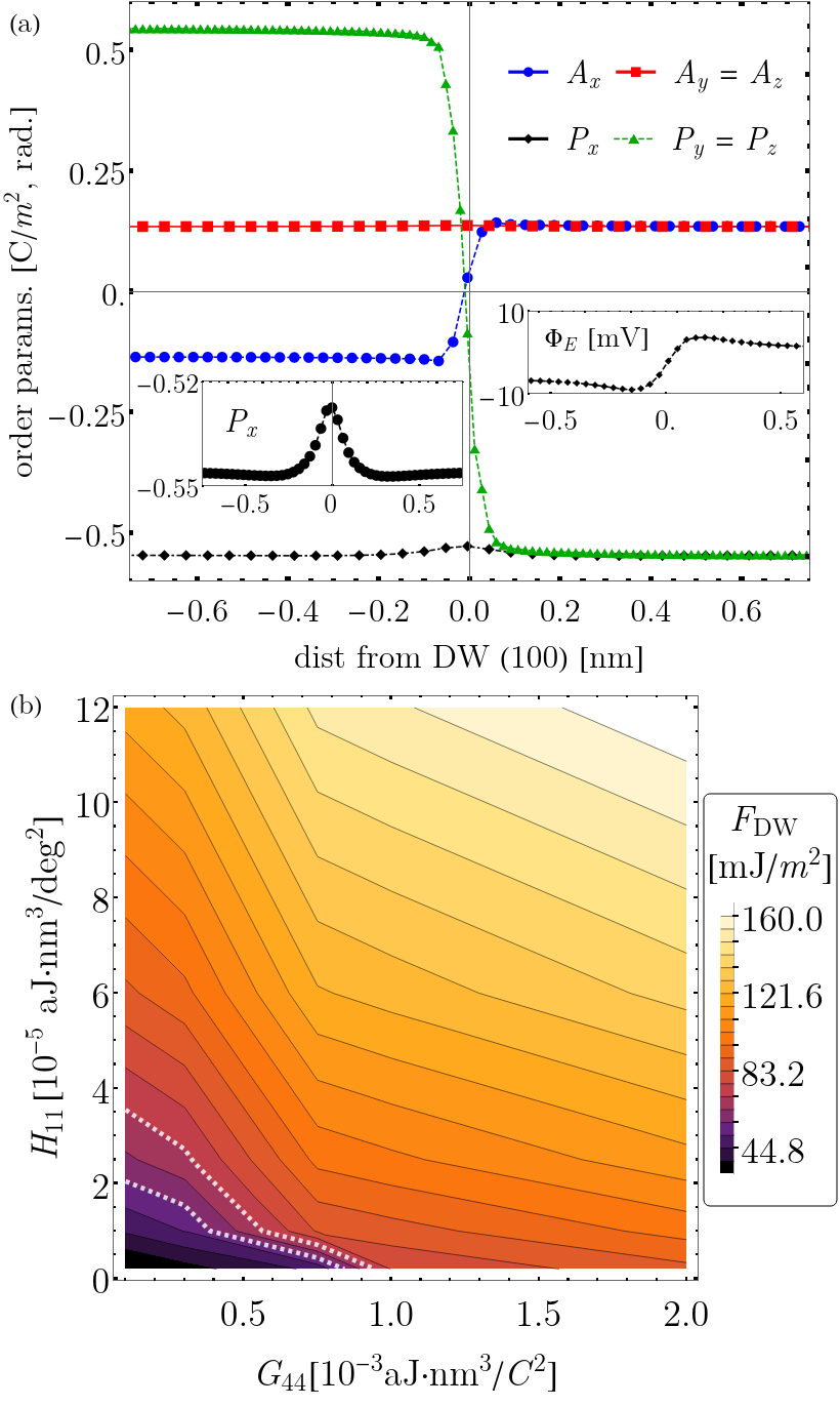
As a first example, consider the lowest energy DW predicted by DFT, the so-called 2/1 (100) DW which is indeed frequently observed in thin film samples of BFO Zhang et al. (2018); Parsonet et al. (2022). The primary gradient coefficients governing the energy of the wall are the and coefficients owing to the fact that , , and are nonzero (see Table 1). The resulting DW profile for the 2/1 (100) wall is presented in Fig. 1(a). The profile is a smooth rotation of both and across the wall region. The inset on the left reveals that the non-switching component experiences a slight decrease () at the wall. The quantitative value of the modulation of the non-switched component is consistent with DFT results of the same DW typeKörbel and Sanvito (2020).
The small change of corresponds with a built-in shown in the right inset panel which is of comparable order ( mV) to those estimated from DFTKörbel and Sanvito (2020). Fitting the - profile shows that the DW is quite thin (thickness nm). Hence, we obtain DWs with marked Ising character. We provide an energy profile scan across the primary coefficients and in (b). The dashed white line outlines the predictions from DFT results in Ref. [(40)]. We also should mention that the dependence on other coefficients is quite weak due to the relatively small gradients in non-switching components. These calculations (and others not shown here) reveal that the choice of is not unique, i.e. one can find the same DW energies (with very similar profiles) for different combinations of the primary coefficients. Therefore, it is necessary to visit other DW configurations to constrain the values of the entire set.
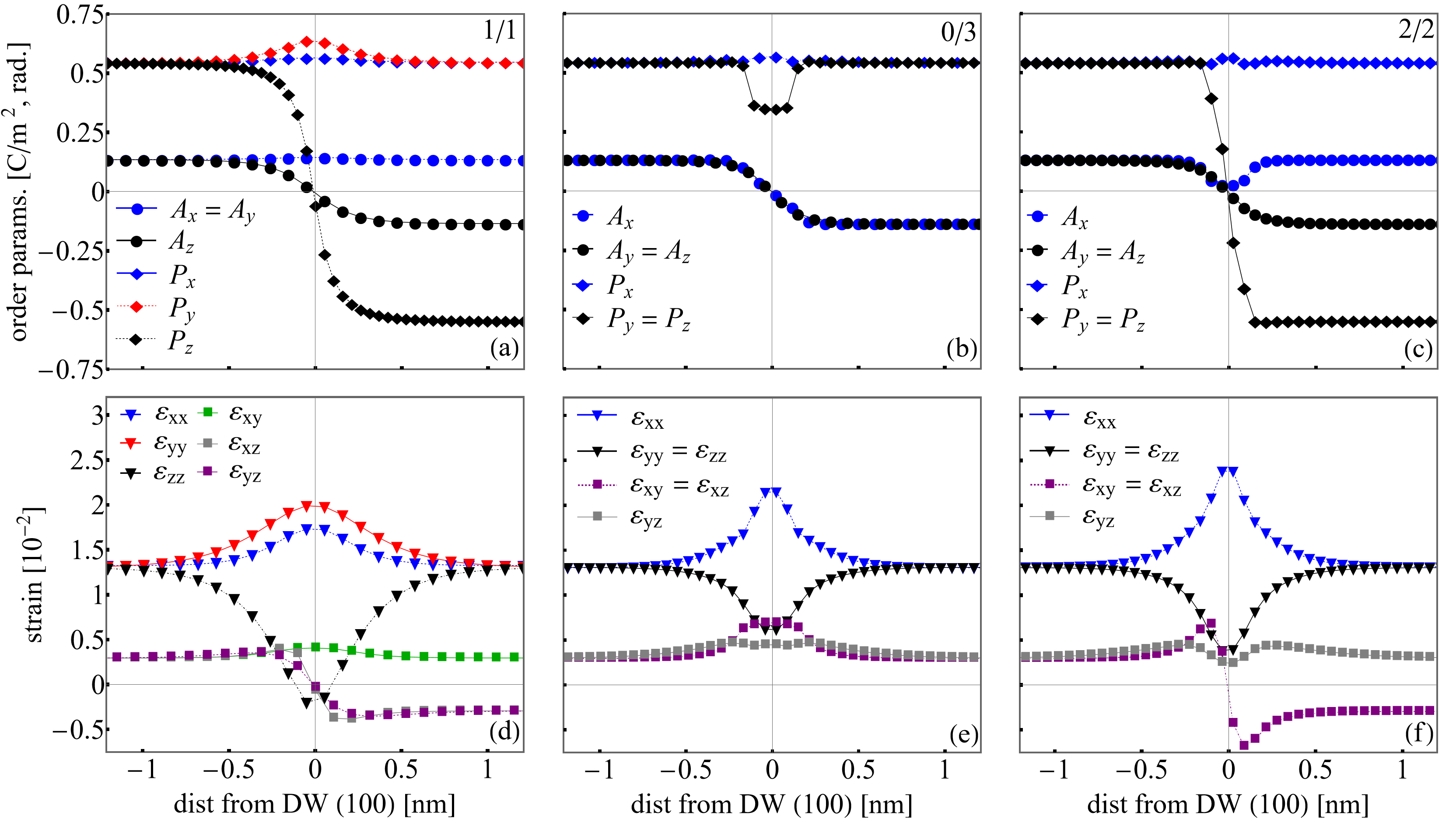
Next, we present - profiles of three higher energy (100)-oriented domain walls (1/1, 0/3, and 2/2) in Fig 2 (a), (b) and (c) respectively. These three calculations correspond to those using our best estimates of the gradient coefficients in Table 2. In all three cases, we find the presence of a small changes in the non-switching components of the order parameters shown in circles for and diamonds for . For example, in the 1/1 shown in DW Fig 2 (a), (in red) which does not change sign, grows at the DW by about 15. This is in contrast to the component (in blue) which only grows by 2.5 demonstrating the influence of the weak built-in field which reduces the magnitude of this component to keep this wall neutral. Similar changes on the order of about 10 are also seen in components shown in blue. This DW-induced change in P seems to be the largest in the 0/3-type DW shown in (b). Due to the influence of built in electric fields from the solution of the Poisson equation (and our best estimates of the anisotropic gradient coefficients), the value of component grows by about 5 whereas the components diminish by almost -35 (shown in black). Again, we also find changes in the non-switching components in the 2/2 wall, with (blue diamonds) growing by about 2; by contrast and decreases by (blue circles).
In panels (d), (e), and (f) of Fig. 2, we depict the corresponding spontaneous strain profiles corresponding to the cases in panels (a), (b), and (c) respectively. Importantly, far from the DW plane, the spontaneous values of the normal (triangles) and shear (squares) components of the strain converge to their respective values of the single domain state. However, the strained state of the DW causes various components of to grow or depress by large percentages to accommodate the electro- and rotostrictive coupling intrinsic in this structure. In the case of the 1/1 DW in (d), the value of the (in black) shrinks until eventually changing sign (smoothly) at the domain boundary. For the 2/2 DW, there is a large tensile strain in (in blue) growing by about a factor of three across the wall.
Also presented in Table 1 are the DW thicknesses associated to the corresponding order parameters, which differ between and . We should note that the thicknesses of the DW corresponding to and differ. This arises because our resulting fit parameters are anisotropic (i.e. ) and also the presence of growth/decrease in non-switching components of and due to the roto- and electrostrictive coupling. Nevertheless, as seen in the table, the domain walls are quite thin ( nm) which agrees quite-well with the available literature on BFO suggesting atomistically thin DWs Diéguez et al. (2013); Hlinka et al. (2017); Körbel and Sanvito (2020); Borisevich et al. (2010). The smaller value of the DW thickness in the (as compared to ) also shows good qualitative agreement with measurements from experiments using Z-contrast scanning transmission electron microscopyBorisevich et al. (2010).
We extend this type of analysis iteratively for the possible DWs listed in Table 1 so that we can converge our set of coefficients yielding reasonable values comparable to DFT; importantly, capturing the energy hierarchyDiéguez et al. (2013); Körbel and Sanvito (2020); Xue et al. (2014) predicted for the collection of walls. Our best estimates of the gradient coefficients found through our fitting procedure are presented in Table 2. We find that in agreement with similar studies on BFOXue et al. (2014, 2021). This is an important relationship that results from harmonic models of antiferrodistortive cubic perovskite materials which has been connected to an asymmetry in the phonon bands at the R pointGesi et al. (1972); Stirling (1972); Cao and Barsch (1990). Another result from our fits is that the energy hierarchy yields for the lowest energy wallsLubk et al. (2009); Diéguez et al. (2013); Xue et al. (2014, 2021).
II.5 Antiferromagnetic energy terms
Now we turn to the AFM order present in BFO. To encapsulate the magnetic behavior of single crystalline BFO, we propose a continuum-approximation to the magnetic free energy density. We consider the total free energy density of the magnetic subsystem () to be a sum of the terms responsible for the nominally collinear AFM sublattices () and those producing the noncollinearity (canted magnetism) by coupling to the structural order (). We first consider the magnetic energy due to the spin subsystem that is not coupled to the structural order,
| (21) | ||||
where controls the strength of the short-range superexchange energy which favors the spins to have collinear AFM ordering Rezende et al. (2019). At our coarse-grained level of theory, we only consider the first nearest-neighbor exchange coupling which has been calculated from first-principles methodsXu et al. (2019) to be approximately 6 meV/f.u. corresponding to in our simulations. The second term describes the AFM non-local exchange stiffness proposed in Ref. [(15)] with meV/nm (or ergs/cm). The third term corresponds to a weak single-ion anisotropy Weingart et al. (2012) with eV/; this term reflects the cubic symmetry of the lattice and breaks the continuous degeneracy of the magnetic easy-plane into a six-fold symmetry.
The remaining terms are due to the magnetostructual coupling,
| (22) |
where
| (23) |
is due to the antisymmetric DMI which acts to break the collinearity by competing energetically with the first term of Eq. (21). It should be emphasized here that the local oxygen octahedral environments of adjacent Fe atoms underpins the DMI vector Ederer and Spaldin (2005); Fennie (2008); de Sousa and Moore (2009); Rahmedov et al. (2012); Meyer et al. (2022). Therefore, the order parameter enables the DMI coupling. Ref. [(13)] provides an estimate of the DMI energy corresponding to eV/f.u. It should be mentioned that the weak canting between and arises from a competition between and and that different estimates of their values can provide the same degree of canting of the sublattices provided they have the same ratio . We come back to this in the next section.
BFO is an easy-plane antiferromagnetDixit et al. (2015), in which the magnetic sublattices lie in a plane defined by the direction of . We include the magnetocrystalline anisotropy termRezende et al. (2019) requisite for easy-plane AFMs as,
| (24) |
with the usual definition of enforcing the easy-plane condition for with . Using DFT methods, Dixit and co-workers Dixit et al. (2015), determined that the relative energy difference between aligning the magnetic sublattices along or in the plane normal to is meV/f.u. Therefore, we choose for our simulations.
We further couple the magnetic energy surface to the structural order by allowing the weak single-ion anisotropy to also depend on the antiphase tilts Weingart et al. (2012) through,
| (25) |
which is in addition to the term in Eq. (21). The choice of and corresponds to a small energy barrier between the 6-fold possible orientations of the weak magnetization thus breaking the continuous degeneracy in the easy-plane. These coefficients can be obtained from DFT calculations as shown in Refs [(13)] and [(41)]. Therefore, we choose our coefficients (see Table 3) such that the relative energy density barrier for the six-fold symmetry is 0.01 meV/ which is a reasonable approximation based on the aforementioned works. We find no influence of this choice of coupling constant on the results presented in this manuscript. The coefficients for and are listed in Table 3.
| 18.7 | Ref. [(15)] | |||||||||||
| -23.4 | Ref. [(42)] | |||||||||||
| 0.0046 | this work | |||||||||||
| 31.25 | Ref. [(13)] | |||||||||||
| 0.0022 | ||||||||||||
| 0.00015 |
We should note that a long-period ( nm) cycloidal rotation of the weak magnetization is often observed in BFO samplesBurns et al. (2020); Agbelele et al. (2017); Xu et al. (2021). It is possible to eliminate the cycloidal order by doping Sosnowska et al. (2002), epitaxial strain Bai et al. (2005); Sando et al. (2013); Burns et al. (2020), applied electric fields de Sousa et al. (2013), or by some processing techniques (i.e. via a critical film thickness) Burns et al. (2020) during synthesis. The spin-cycloid could be incorporated into our model by including coupling terms associated with a proposed spin-current mechanism Agbelele et al. (2017); Popkov et al. (2016); Xu et al. (2022). However, in order to provide the simplest model of the ME multiferroic effects, we have neglected them in this work.
II.6 Micromagnetics and homogeneous spin ground states
In order to find the spin ground states in the presence of an arbitrary structural fields, we consider the Landau-Lifshitz-Bloch (LLB) equation Garanin and Chubykalo-Fesenko (2004) that governs the sublattices ,
| (26) | ||||
where is the phenomenological Gilbert damping parameter and is the electronic gyromagnetic coefficient equal to rad. m A-1 s-1. The effective fields are defined as with the permeability of vacuum. The saturation magnetization density of the BFO sublattices is B/FeWeingart et al. (2012); Xu et al. (2019, 2022). The third term arises from the LLB approximation in the zero temperature limit where is a damping along the longitudinal direction of . We implement the LLB equation as a numerical resource in order to provide a restoring force and bind the quantities to the unit sphere . In this context, we consider our spin subsystem to be at K in results presented throughout in this paper. In the Appendix, we provide a short derivation of the LLB torque in the zero temperature limit. We set in all results in this work to satisfy the constraint on .
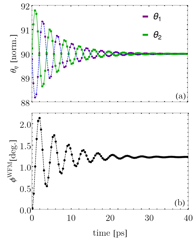
To look for homogeneous spin ground states, we consider and evolve Eq. 26 (utilizing the numerical approach described in Sec. II.3) until the relative change in the total energy computed from the summation of Eq. (21) and Eq. (22) between adjacent time steps is eV/s. Also, we stress that the influence of is negligible in all results presented in this work provided that its unitless value is around or above. To verify that our ground states predict the magnetic ordering consistent with the literature of BFO, we define two angular variables and . The former tracks the degree of canting between the sublattices and the latter tracks the orientation of the magnetization with respect to , the magnetic easy-plane normal. As an example, we first set along the [111] direction to be static. The time evolution (ringdown) of Eq. (26) is highlighted in Fig. 3(a) for showing that the sublattices have relaxed into the easy plane defined by with In (b) the time dependence of the canting angle during the relaxation is shown. At the conclusion of the ringdown, reaches a value of . This demonstrates that the angular quantities detail an orthogonal system of the vectors as often discussed in the literature Heron et al. (2014).
| (): | ||||||||||||||||
|---|---|---|---|---|---|---|---|---|---|---|---|---|---|---|---|---|
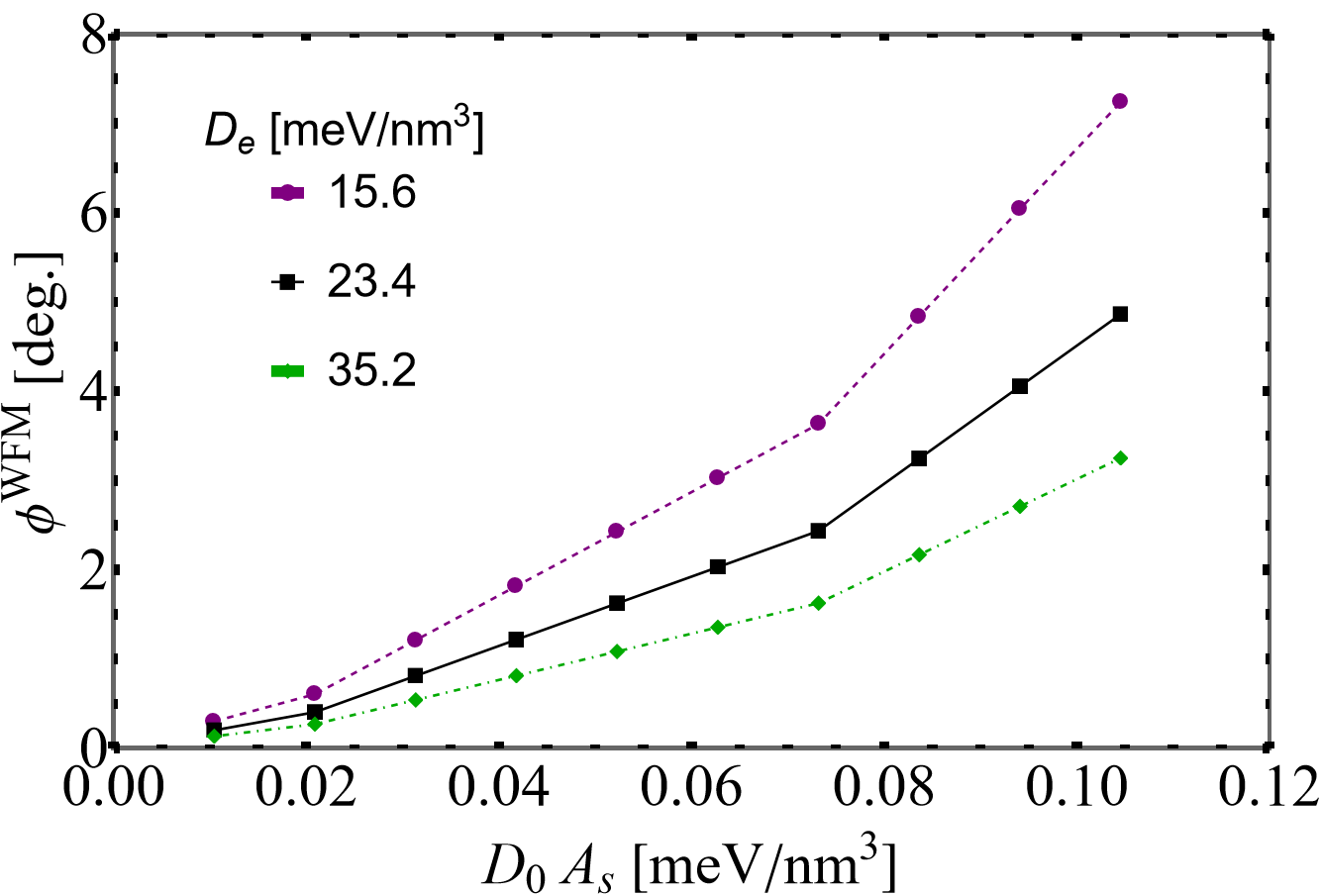
As a further benchmark, we probe the influence of the ratio on the values of . This test, shown in Fig. 4 highlights the energetic competition between the AFM superexchange and the sublattice DMI. From Ref. [(42)] we have meV/nm3 and our analysis demonstrates provided meV/nm3. We thus have the weak moment B/Fe, which agrees well with the available literature Wojdeł and Íñiguez (2010); Tokunaga et al. (2010); Dixit et al. (2015); Xu et al. (2019).
By setting along the eight polar directions possible in BFO, we can find six magnetic states for each of them. The corresponding 48 multiferroic domains are listed in Table 4. For all orientations calculated, the canted angle is precisely . Additionally, when is reversed fully (), which is an acceptable ground state in our potential, the sign of will change but not the sign of the Néel vector . Hence, we have a total of 96 possible domain variants. Due to the DMI these quantities listed in this table are canted slightly from their listed values (hence the use of symbol).
II.7 Antiferromagnetic domain walls
Using low-energy electron microscopy (X-PEEM), AFM domain boundary contrast can be visualizedMoubah et al. (2012) within a single ferroelectric domain. To better understand the capabilities of our modeling effort, we attempt to stabilize an AFM DW (i.e., one with switched ) corresponding to the above experimental observations. We set along to be homogeneous (and fixed in time) within the computational box. Then, a sin(x) profile is chosen for the sublattices corresponding to two possible Néel orientations of Table 4 for a (100)-oriented domain boundary with homogeneous . After relaxation Eq. (26) with large Gilbert damping , we find that the AFM wall is not stable and the system evolves to a homogeneous state with corresponding to one of the six possible orientations allowed in the domain. If the non-local exchange interaction governed by Agbelele et al. (2017) is reduced by a factor of ten, then we find that the solution corresponds to AFM domain walls with a rotation of , i.e and . We estimate that the corresponding DW in has a characteristic width of 20 nm and a corresponding DW energy of mJ/ using Eq. (20).
Let us now consider how the structural DWs affect the net magnetization. The modulation of and across the domain boundary drastically alters the magnetostructural coupling energy surface due to Eq. (22) causing the AFM order to choose preferential orientations associated with those calculated in Table 4. Careful inspection of Table 4 suggests that only certain low energy magnetic DWs (i.e., those minimizing the gradient of ) should be observed for the different FE domain walls listed in Table 1. Using our previously established notation for adjacent DW states, the lowest energy FE DW (2/1) corresponding to a to change will only allow or and or respectively with no changes to the Néel vector . This coincides with a rotation of consistent with a change of the oxygen octahedral tilt field albeit having a switch.
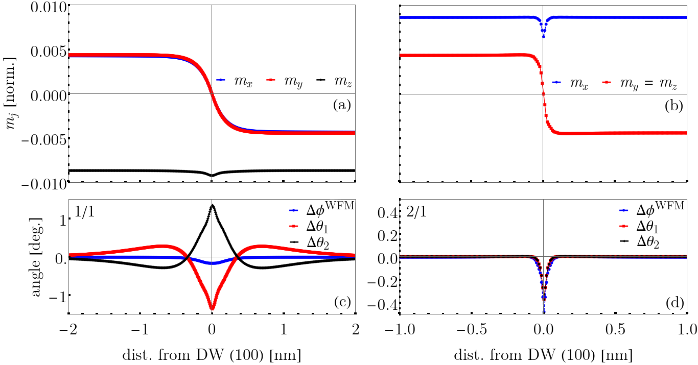
To calculate the magnetic textures numerically, we fix in time the FE order parameters - corresponding to a specific DW in Sec. II.4. We choose the 1/1 (100) and 2/1 (100) structural walls as they are most commonly observed in experiment. Again, we use a large Gilbert damping and look for the ground states utilizing Eq. (26). In Fig. 5, we display the weak moment as a function of the distance to the DW plane for the 1/1 (a) and 2/1 (b) walls after relaxation. In both cases, the rotates by - to in (a) and to in (b) - with a sharp interface region. This is expected as the DMI term is driven by the vector forcing to also change by . The large value of causes the Néel vector to be nearly constant across the DW corresponding to in (a) and in (b) as it satisfies both conditions of the ground state in adjacent domains. Fitting the switched components of to the aforementioned tanh(x) profile from Sec. II.4 yields nm. We can calculate a thickness of nm in the 2/1 (100) case demonstrating a nearly atomistically thin DW in the magnetic texture. A comparison to Table 1 shows that we have an equality of in both 1/1 (100) and 2/1 (100) walls.
The component of that does not switch, black in (a) and blue in (b), changes by about and respectively across the DW region indicating rotational components of . This leads to a deviations of the angular quantities from their ground state values. We plot these quantities in panels (c) and (d) of Fig. 5. We see that, in the 1/1 (100) case in (c), the sublattices cant slightly () out of the easy plane to facilitate this magnetic reversal. The weak magnetization canting angle (shown in blue) also reduces its magnitude by about . This is different from the behavior of the angular quantities of the 2/1 (100) DW shown in panel (d) which decrease their values by about in the same fashion indicating canting out of the easy-plane in the same direction for both sublattices resulting in a slight reduction of . We stress that these quantities should be meaningful since they are on the order of in the ground state and that in the 1/1 (100) case, the modulations extend more than a few unit cells from the DW ( nm).
By using Eq. (20), we can estimate the energy of the magnetic DW of the 1/1 (100) and 2/1 (100) cases. For the 1/1 and 2/1 walls, we calculate and mJ/ respectively. The energy difference between these two DWs is quite small despite having a very different profile of and . The variation of in panel (c) for the 1/1 (100) case causes a large relative increase in the easy-plane anisotropy for both sublattice contributions as compared to (d) for the 2/1 (100) DW. However, as seen in the panel (d), there is more identifiably sharp structure (i.e., modulations of and occur within nm of the DW) as switches by . This leads to an increase in the DMI energy relative to the 1/1 case. We have only presented data on these two types of magnetic boundaries in the presence of the - DWs. Higher energy DWs can also be investigated with our approach, but we leave this for future work.
III Applications: spin waves and magnetoelectric switching
III.1 Spin waves through multiferroic domain boundaries
The field of spintronics relies on the generation, control, and read-out of traveling packets of spinHirohata et al. (2020). In AFMs, the spin precessional processes can occur at low energy and ultrafast frequencies (THz and above) thus leading to competitive advantages in information processing design as compared to standard CMOS technologyJungwirth et al. (2016); Baltz et al. (2018). The basic concept of wave transmission and reflection phenomena is key to understanding how to optimize spin wave transport in these systems. Recently, researchers established non-volatile control of thermal magnon transport in BFO using electric fields Parsonet et al. (2022). Their work demonstrates that the FE DWs act as a barrier to spin transport across a length-scale comprising many 100s of nm and dampen the detected magnon signal useful for the device. We will illustrate the usefulness of our approach by showing how it can enable a mesoscopic simulation of this situation
We consider the two of the commonly observed DWs in BFO experiments, the 2/1 and 1/1 (100)-oriented boundariesHeron et al. (2014); Johann et al. (2012); Parsonet et al. (2022). The reader is referred to Table 1 and the previous section for the initial conditions of the order parameters. There is a large relative difference between the lattice and spin DW energies. This suggests that any application of an external magnetic field should not appreciably influence the and subsystem. Therefore, we fix in time the structural order parameters in this section. We couple to act on the net magnetization through the Zeeman free energy density,
| (27) |
and add it to the total free energy of the spin configuration.
In order to perturb the system, we consider gaussian spin wave beams generated by a field of the form Gruszecki et al. (2015),
where field amplitude kOe, excitation location , gaussian intensity profile parameter , and control the perturbation distribution in spacetime. The director orients the magnetic field with respect to . Finally, we cut-off the pulse at ps and excite the spin waves at a frequency .
Eq. (26) is evolved with and Eq (III.1). We enforce periodicity in our computational volume along the for the and variables. The time-integration of Eq. (26) is set for fs time steps to ensure numerical convergence for the fast AFM dynamics in the system. We verify that our calculations are in the linear limit by adjusting the and determine that the perturbed amplitudes of scale linearly. Finally, we monitor the system total free energy and (via the LLB term) and verify that they are constant to within floating point accuracy for all time in our simulation.
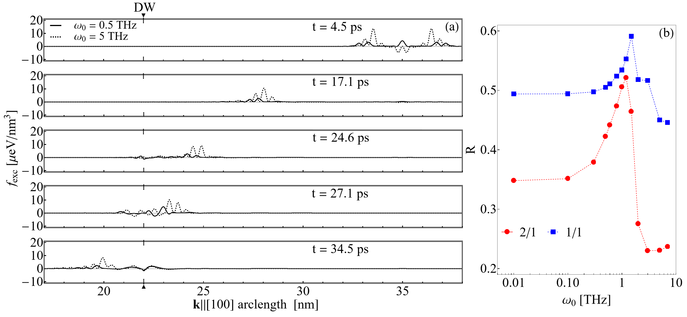
In Fig. 6(a), we track the excess free energy density . Therefore, corresponds to a small energy that is injected into our computational volume by the spin excitation at time . A few snapshots of the due to the propagating wavefront (at two different ) are presented in Fig. 6(a) in sequential panels from top to bottom for , and ps. Here in panel (a), the DW is marked at nm and is impacted by the spin wave at around ps. The excess energy density loss after the wavefront travels through the DW can be calculated by numerically time integrating at distances of nm left and right from the DW plane located at .
We then compute their ratio ,
| (28) |
to determine which percentage of the excess energy due to the incoming wave is reflected or absorbed by the DW, i.e., the degree of rectification. We see in Fig. 6(b) that varies substantially across several decades in frequency with an asymptote for low frequencies corresponding to about 35 and 50 rectification for the 2/1 and 1/1 walls respectively. The relative difference between rectification arises from the excitation of the DW region by the spin wave (seen in Fig. 6(a) for ps). To verify this, we track the time integrated at the DW revealing almost all of the excess energy is absorbed by the DW. In this analysis, we find that only a small portion of due to this spin wave is reflected (not shown). When the frequency is increased, a maximum in DW excess energy absorption in is acquired around 1-2 THz before abruptly decreases indicating that the DW becomes more transparent to the spin wave. Similar frequency-dependent transmission ratios have been reported in the literature for noncollinear AFMsRodrigues et al. (2021). We should mention that we did not find any meaningful influence of or on our results except changing the relative rectification between the two types of walls, but a more detailed study of the parameters is warranted.
Finally, we should comment on how this agrees with experimental observations. In the work of Parsonet et alParsonet et al. (2022), the propagating thermal magnon signal inferred from the inverse spin Hall effect was seen to decay exponentially as a function of distance from the source. This was postulated as due to the 2/1 (100)-oriented DWs in the system acting as a barrier to spin currents with whose number increased upon electrode separation; we can conclude that our results support this conclusion qualitatively. It remains to be seen if domain engineering techniques guided by similar calculations could possibly help control the rectification that impedes efficient control of magnon signals in ME spintronics. Also, we should mention that as opposed to our approach detailed in this section, in principle and could vary in time. This would lead to electromagnonic effects localized to the DWs upon excitation of inhomogeneous magnetic and/or electric fields (as highlighted in recent Refs. [(86; 87)]). It is possible that the coupled vibrations of the structural order could further influence the spin transport. However, this is a outside the scope of this work and warrants future studies.
III.2 Magnetoelectric switching of the AFM order
A considerable demand in AFM spintronics is to find an adequate approach to manipulate the magnetic order with external stimulii. In the case of BFO, since this material displays an intrinsic electric dipole moment, it has been proposed to use an electric field to manipulate and control the magnetic texture. The technological benefits to the prospect of electric field control of magnetism has been considered for some time Heron et al. (2014); Matsukura et al. (2015); Song et al. (2017); Liu et al. (2021); Parsonet et al. (2022). While low-frequency deterministic switching of with an electric field has been experimentally demonstratedHeron et al. (2014), the dynamical processes of the coupled polar-magnetic order is still a topic of researchLiao et al. (2020a, b). We aim to highlight one such use of this modeling effort for the case of ME switching (i.e., using an electric field to switch ).
We now consider a fully-dynamical simulation where all system variables , depend on time. As we are now interested in real dynamics, the time relaxation constants and in Eq. (10) and (11) are taken from Ref. [(91)]. For our switching simulations, our initial condition of the system is along the direction and homogeneous. Since this is a homogeneous calculation, this can be considered the macrospin limit of Eq. (26). Since the dynamics of the AFM order are in general very fast (characteristic frequencies of s of GHz to the THz regime)Jungwirth et al. (2016), we introduce a time stepping constraint on the evolution of Eq. (26) for dt ps to ensure numerical convergence. There is no spin dissipation from conduction electrons in BFO due to its insulating nature. Therefore, we choose of order which is a reasonable assumption for BFO Wang et al. (2012); Bhattacharjee et al. (2014) and other magnetic insulators Kapélrud and Brataas (2013); Shiino et al. (2016); Soumah et al. (2018); Chen and Dong (2021).
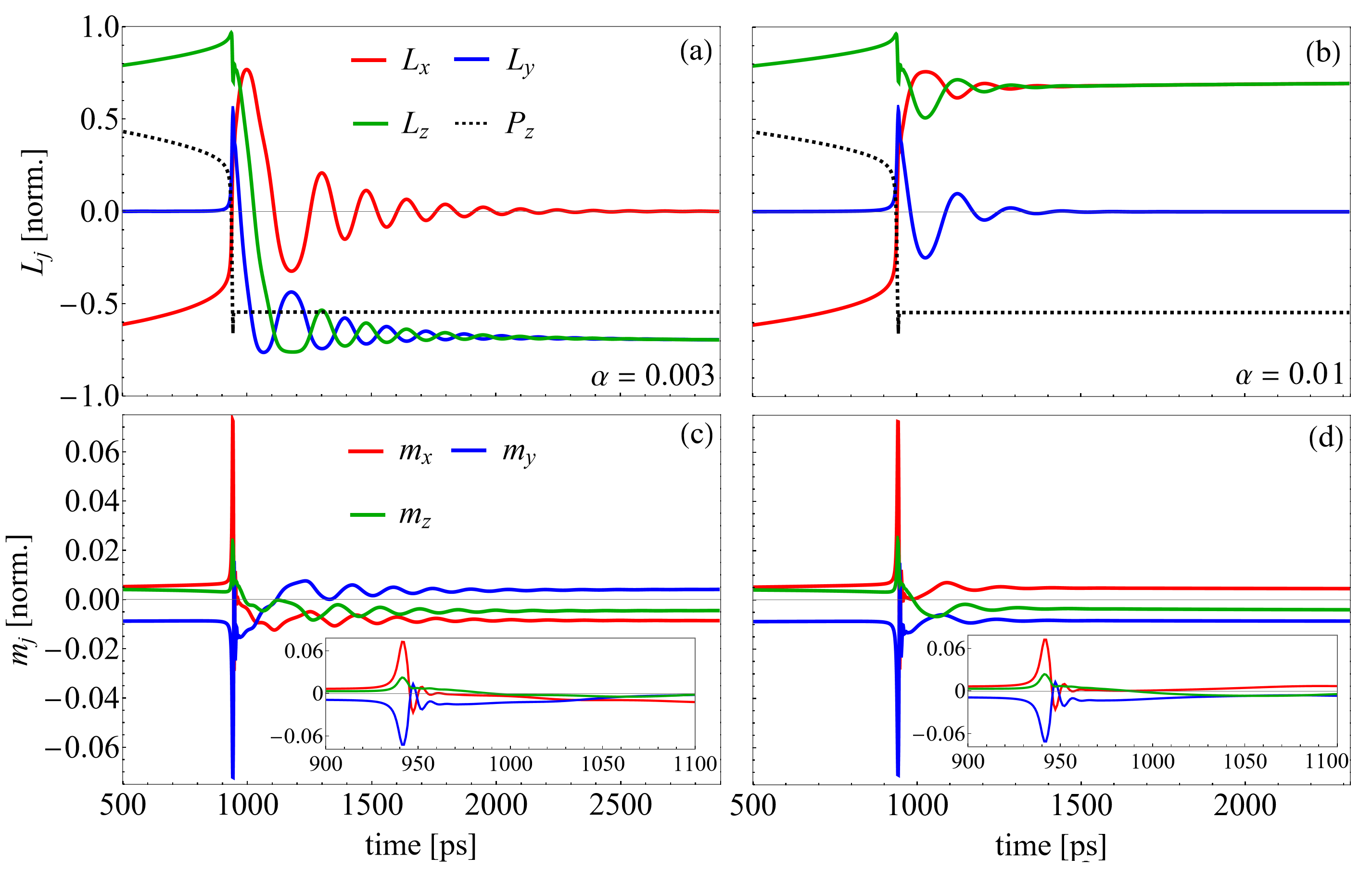
As one example to switch the component of , we choose our electric field to be with MV/m. This is a large value compared to coercive fields of MV/m observed in switching experiments of thin film BFO heterostructuresWang et al. (2003); Heron et al. (2014). However, it is well-known that the coercive field needed to fully switch components of in perovskite FEs is intrinsically linked to the occurence of various phenomenaMorozovska (2005); Bratkovsky and Levanyuk (2000); Indergand et al. (2020); Gerra et al. (2005); Liu et al. (2016) that are not present in our homogeneous switching simulations. We select an E frequency of MHz. The field is abruptly turned off after has switched in order to facilitate only one switching event for analysis. The initial state is homogeneous along [111] with and as one of the possibilities listed in Table 4. In order to investigate if the ME switching has dependency on , we pick two different values and and evolve Eq. (10) and (11) in the presence of the field.
Here we see in Fig. 7(a) and (b), the application of along the direction switches the (and also , not shown) orientation to within ps (dashed black line). We use the notation to denote initial states and final states for the system. The change of the energy surface through the magnetostructural coupling causes to switch orientation from to in (a) and in (b). At the same time, the direction of undergoes and transitions in (c) and (d). When one compares the dynamics between the left and right panels of Fig. 7, it is evident that the choice of influences the final state despite having nearly identical ringdown patterns at the temporal vicinity of the switch shown in the insets of (c) and (d). Shortly after the switch ( ps), the magnetization evolves differently, due to different maximum amplitudes, leading to transition pathways which overcome different energy barriers.
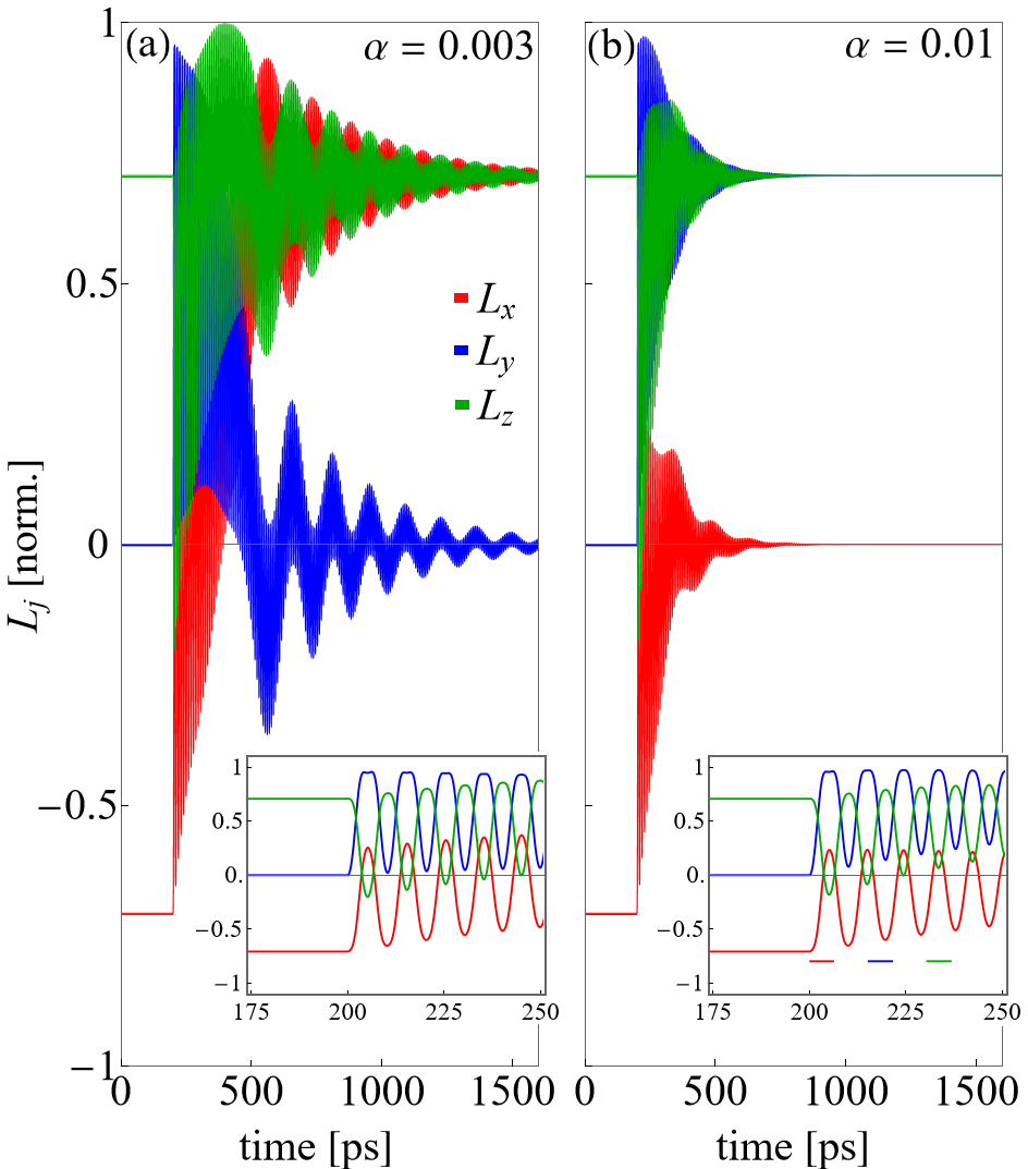
We also consider an instantaneous limit of the switching process where the is switched immediately. In Fig. 8(a) and (b) which correspond to the same values as in 7(a) and (b), the switch is set to occur at ps (shown in the insets). The relaxation of Eq. (26) with the damping set to and creates many oscillations with a characteristic ringdown frequency of approximately GHz. We find that indeed, the same situation happens presented in Fig. 8(a) and (b) as in Fig. 7(a) and (b) with the final states of determined by its initial orientation and the final configuration of . The vector (not shown) has trajectories and in Fig. 8(a) and (b) respectively. In the simulations corresponding to Fig. 7, the switching of occurs in about a 200 ps time window, whereas with the instantaneous calculation, the switching pathway requires at least 1 ns to ring down with realistic material values of . This is far above the theoretical switching limit of 30 ps proposed by Liao and co-workersLiao et al. (2020a, b) who also utilized a LLG model for the AFM order coupled to a Landau-type parameterization.
We stress that both of these numerical simulations are exercises for illustrative purposes and are simplified versions of the dynamic processes that would happen in an experiment. Our calculations already suggest two things: (1) the Gilbert damping controls the maximum amplitude of the oscillations and thus the final state, hence it needs to be understood in BFO to have a repeatable effect and that (2) the dynamics of the structural switching does not seem to be essential in controlling the switching pathway (i.e. comparing the explicit time dependent calculations vs, the instantaneous - switches). A more detailed investigation remains for the future.
IV Conclusions and outlook
We have presented a continuum model for BFO able to treat the polar, octahedral tilt, spontaneous strain, and the AFM order in a single calculation. This model is built upon micromagnetic and FE phase field approximations to the system order parameters. Our model is benchmarked against the known behavior in this material - specifically, we have parameterized the FE DW profiles along with their spontaneous strain fields obtaining an energy hierarchy of possible states in agreement with DFT calculationsDiéguez et al. (2013). We also provide simulations of in the presence of low energy FE DWs revealing delicate features in the angular quantities characterizing the canted magnetism. Next, we illustrated the usefulness of the model with two simple applications i) AFM spin waves traversing the multiferroic domain boundary highlighting a rectifying nature in qualitative agreement with recent experiments Parsonet et al. (2022) and ii) fully-dynamical ME switching in real-time which, interestingly, reveals a sensitivity of switching pathways on the Gilbert damping.
There are many other phenomena in BFO that could be built upon our model. As is often discussed in the literature regarding BFO, is the appearance of a long-period spin cycloid Agbelele et al. (2017); Burns et al. (2020) in which the proposed origin is underpinned by an asymmetric spin-current mechanismGareeva et al. (2013); Popkov et al. (2016); Xu et al. (2021); Meyer et al. (2022) which is necessary to stabilize these patterns. While the results of this paper are for the weakly non-collinear AFM order, one can appreciate that the presence of the spin cycloid might affect the outcome of our illustrative examples. We also emphasize that the DMI expression in Eq. (23) is isotropic and that the application of strain should break the symmetry which can lead to different AFM sublattice ordering as detailed in Ref. [(13)]. In principle, both the spin-flexoelectric (spin cycloid) and magnetoelastic (epitaxial strain) contributions could influence the antisymmetric exchange leading to drastically altered magnetization textures in the simulations. In general also, this type of multiferroic modeling could be extended to other noncollinear antiferromagnets such as those where electric fields have been shown to manipulate the magnetic state despite lack of spontaneous FE orderHe et al. (2010); Kosub et al. (2017).
The model is built within the Ferret Mangeri et al. (2017) module atop the open-source Multiphysics Object Oriented Simulation Environment (MOOSE) framework Permann et al. (2020). As a nod to open-science, we provide representative examples for all of the results in this paper to be hosted on a GitHub websiteFer (2023). Ferret is part of a forward-integrating toolset called the Continuous Integration, Verification, Enhancement, and Testing (CIVET) Slaughter et al. (2021) utility which preserves reproducibility of our results by ensuring underlying code changes to the MOOSE software stack do not break the module. The sets of governing equations and energy terms in this paper, which are applicable in 3D and for any geometry, are available and documented as C++ objects within the open-source software repository. While our modeling effort is certainly not exhaustive, we believe it will be a useful platform for development of continuum simulations of BFO and other multiferroics in length and time-scales are not accessible by atomistic methodologies.
Acknowledgements.
The authors thank Natalya Fedorova for valuable input. J. M. has received funding from the European Union’s Horizon 2020 research and innovation programme under the Marie Skłodowska-Curie grant agreement SCALES - 897614. Work by O.H. supported by Basic Energy Sciences Division of the Department of Energy. D.R.R. acknowledges funding from the Ministerio dell’Università e della Ricerca, Decreto Ministeriale n. 1062 del 10/08/2021 (PON Ricerca e Innovazione).Appendix
In micromagnetic simulations in which thermal fluctuations are not included (so-called athermal simulations), the magnetization density must remain constant in magnitude, thus preserving the unit norm of the magnetization director . In finite-difference codes on regular meshes, such as MuMax3Vansteenkiste et al. (2014), enforcing this constraint is simple: each simulation cell contains one unit vector that can simply be renormalized after, e.g., each time step. In contrast, in weak-formulation FEM codes the continuum magnetic degrees of freedom are approximated by shape functions on irregular mesh cells and integrated over, and normalization of is not as easily interpreted or made meaningful as in finite-difference codes.
One can overcome this problem, for example using, a representation of in spherical coordinatesYi and Xu (2014), but numerical solutions of the equations of motion can become unstable leading to serious convergence issues. Another possibility is to introduce the constraint through a Lagrangian multiplier or using special shape functions on the tangent plane of the magnetization director vector fieldAlouges and Jaisson (2006); Szambolics et al. (2008). We chose a different path, which is physically grounded in the Landau-Lifshitz-Bloch (LLB) formulationGaranin (1997); Garanin and Chubykalo-Fesenko (2004); Evans et al. (2012). The key point in the LLB formulation is that longitudinal fluctuations in the magnetization director are allowed, but countered by a penalty for deviations away from the thermodynamic average of the magnitude at a temperature . The longitudinal fluctuations add a term to the equation of motion that is given by
| (29) |
where is the local magnetization director with an equilibrium value that depends on temperature, is a thermal field, and is the usual dimensionless Gilbert damping. The longitudinal damping depends on through
| (30) |
with the mean-field Curie temperature, and the effective field includes the longitudinal susceptibility ,
| (31) | |||||
Here , , and are the usual external, anisotropy, and exchange fields. Ignoring the thermal field, the contribution to is then
| (32) |
At with we can simplify the last term in the above equation to get
| (33) |
where now has the unit of a magnetic field that drives the longitudinal relaxation. The contribution to the time evolution of due to longitudinal relaxation is then
| (34) |
One can show that in the limit of low , much lower than relevant Curie temperatures, the second term in Eq. (34) can be ignored. In this case, the LLB-like addition to the equations of motion is simply
| (35) |
where has the dimension of a field.
References
- Scott (1974) J. F. Scott, Reviews of Modern Physics 46, 83 (1974).
- Rabe et al. (2007) K. Rabe, C. H. Ahn, and J.-M. Triscone, Physics of Fer- roelectrics: A Modern Perspective (Springer-Verlag Berlin Heidelberg, 2007).
- Stöhr and Siegmann (2006) J. Stöhr and H. C. Siegmann, Magnetism: From Fundamentals to Nanoscale Dynamics (Springer, 2006).
- Kézsmárki et al. (2015) I. Kézsmárki, S. Bordács, P. Milde, E. Neuber, L. M. Eng, J. S. White, H. M. Rø nnow, C. D. Dewhurst, M. Mochizuki, K. Yanai, H. Nakamura, D. Ehlers, V. Tsurkan, and A. Loidl, Nature Materials 14, 1116 (2015).
- Heron et al. (2014) J. Heron, J. Bosse, Q. He, Y. Gao, M. Trassin, L. Ye, J. Clarkson, C. Wang, J. Liu, S. Salahuddin, D. Ralph, D. Schlom, J. Iniguez, B. Huey, and R. Ramesh, Nature 516, 370 (2014).
- Lin et al. (2017) L.-F. Lin, Q.-R. Xu, Y. Zhang, J.-J. Zhang, Y.-P. Liang, and S. Dong, Physical Review Materials 1 (2017).
- Seki et al. (2009) S. Seki, H. Murakawa, Y. Onose, and Y. Tokura, Physical Review Letters 103, 237601 (2009).
- Fiebig et al. (2016) M. Fiebig, T. Lottermoser, D. Meier, and M. Trassin, Nature Reviews Materials 1 (2016).
- Spaldin and Ramesh (2019) N. A. Spaldin and R. Ramesh, Nature Materials 18, 203 (2019).
- Moreau et al. (1971) J. Moreau, C. Michel, R. Gerson, and W. James, Journal of Physics and Chemistry of Solids 32 (1971).
- Smith et al. (1968) R. T. Smith, G. D. Achenbach, R. Gerson, and W. J. James, Journal of Applied Physics 39 (1968).
- Ederer and Spaldin (2005) C. Ederer and N. A. Spaldin, Physical Review B 71, 060401 (2005).
- Dixit et al. (2015) H. Dixit, J. Hee Lee, J. T. Krogel, S. Okamoto, and V. R. Cooper, Sci. Rep. 5 (2015).
- Sando et al. (2013) S. Sando, A. Agbelele, D. Rahmedov, J. Liu, P. Rovillain, C. Toulouse, I. C. Infante, A. P. Pyatakov, S. Fusil, E. Jacquet, C. Carrétéro, C. Deranlot, S. Lisenkov, D. Wang, J.-M. Le Breton, M. Cazayous, A. Sacuto, J. Juraszek, A. K. Zvezdin, L. Bellaiche, B. Dhkil, A. Barthélémy, and M. Bibes, Nature Materials 12, 641 (2013).
- Agbelele et al. (2017) A. Agbelele, D. Sando, C. Toulouse, C. Paillard, R. D. Johnson, R. Rüffer, A. F. Popkov, C. Carrétéro, P. Rovillain, J.-M. Le Breton, B. Dkhil, M. Cazayous, Y. Gallais, M.-A. Méasson, A. Sacuto, P. Manuel, A. K. Zvezdin, A. Barthélémy, J. Juraszek, and M. Bibes, Adv. Mater 29 (2017).
- Burns et al. (2020) S. R. Burns, O. Paull, J. Juraszek, V. Nagarajan, and D. Sando, Advanced Materials 32 (2020).
- Xu et al. (2021) B. Xu, S. Meyer, M. J. Verstraete, L. Bellaiche, and B. Dupé, Physical Review B 103, 214423 (2021).
- Manipatruni et al. (2019) S. Manipatruni, D. E. Nikonov, C.-C. Lin, T. A. Gosavi, H. Liu, B. Prasad, Y.-L. Huang, E. Bonturim, R. Ramesh, and I. A. Young, Nature 565, 35 (2019).
- Parsonet et al. (2022) E. Parsonet, L. Caretta, V. Nagarajan, H. Zhang, H. Taghinejad, P. Behera, X. Huang, P. Kavle, A. Fernandez, D. Nikonov, H. Li, I. Young, J. Analytis, and R. Ramesh, Physical Review Letters 129, 087601 (2022).
- Béa et al. (2006) H. Béa, M. Bibes, S. Cherifi, F. Nolting, B. Warot-Fonrose, S. Fusil, G. Herranz, C. Deralot, E. Jacquet, K. Bouzehouane, and A. Barthélémy, Applied Physics Letters 89 (2006).
- Fusil et al. (2014) S. Fusil, V. Garcia, A. Barthélémy, and M. Bibes, Annual Review Materials Research 44, 91 (2014).
- Yin et al. (2018) L. Yin, X. Wang, and W. Mi, Journal of Applied Physics 123, 033905 (2018).
- Takahasi et al. (2006) K. Takahasi, N. Kida, and M. Tonouchi, Physical Review Letters 96, 117402 (2006).
- Guzelturk et al. (2020) B. Guzelturk, A. B. Mei, L. Zhang, L. Z. Tan, P. Donahue, A. G. Singh, D. G. Schlom, L. W. Martin, and A. M. Lindenberg, Nanoletters 20, 145 (2020).
- Paull et al. (2022) O. Paull, C. Xu, X. Cheng, Y. Zhang, B. Xu, K. P. Kelley, A. de Marco, R. K. Vasudevan, L. Bellaiche, V. Nagarajan, and D. Sando, Nature Materials 21, 74 (2022).
- Heo et al. (2022) Y. Heo, H. Zhang, and M. Alexe, Advanced Electronics Materials 8 (2022).
- Lejman et al. (2014) M. Lejman, G. Vaudel, I. C. Infante, P. Gemeiner, V. E. Gusev, B. Dkhil, and P. Ruello, Nature Communications 5 (2014).
- Zhu et al. (2016) M. Zhu, Z. Du, Q. Liu, B. Chen, S. H. Tsang, and E. H. Tong Teo, Applied Physics Letters 108, 233502 (2016).
- Sando et al. (2014) D. Sando, P. Hermet, J. Allibe, J. Bourderionnet, S. Fusil, C. Carrétéro, E. Jacquet, J.-C. Mage, D. Dolfi, A. Barthélémy, P. Ghosez, and M. Bibes, Physical Review B 89 (2014).
- Gross et al. (2017) I. Gross, W. Akhtar, V. Garcia, L. J. Martínez, S. Chouaieb, K. Garcia, C. Carrétéro, A. Barthélémy, P. Appel, P. Maletinsky, J.-V. Kim, J. Y. Chauleau, N. Jaouen, M. Viret, M. Bibes, S. Fusil, and V. Jacques, Nature 549, 252 (2017).
- Chauleau et al. (2019) J.-Y. Chauleau, T. Chirac, S. Fusil, V. Garcia, W. Akhtar, J. Tranchida, P. Thibaudeau, I. Gross, C. Blouzon, A. Finco, M. Bibes, B. Dkhil, D. D. Khalyavin, P. Manuel, V. Jacques, N. Jaouen, and M. Viret, Nature Materials 19, 386 (2019).
- Fusil et al. (2022) S. Fusil, J.-Y. Chauleau, X. Li, J. Fischer, P. Dufour, C. Léveillé, C. Carrétéro, N. Jaouen, M. Viret, A. Gloter, and V. Garcia, Adv. Electron. Mater. 8 (2022).
- Park et al. (2013) M. Park, K. No, and S. Hong, AIP Advances 3 (2013).
- Ivanov (2005) B. Ivanov, Low Temperature Physics 31 (2005).
- Chen (2008) L.-Q. Chen, Journal of the American Ceramic Society 91, 1835 (2008).
- Xue et al. (2021) F. Xue, T. Yang, and L.-Q. Chen, Physical Review B 103, 064202 (2021).
- Liao et al. (2020a) Y.-C. Liao, D. E. Nikonov, S. Dutta, S.-C. Chang, S. Manipatruni, I. A. Young, and A. Naeemi, IEEE Transactions on Magnetics 56, 1 (2020a).
- Liao et al. (2020b) Y.-C. Liao, D. E. Nikonov, S. Dutta, S.-C. Chang, C.-S. Hsu, I. A. Young, and A. Naeemi, Nano Letters 20, 7919 (2020b).
- Govinden et al. (2022) V. Govinden, P. R. Tong, X. Guo, Q. Zhang, S. Mantri, S. Prokhorenko, Y. Nahas, Y. Wu, L. Bellaich, H. Tian, Z. Hong, D. Sando, and V. Nagarajan, arxiv:2209.08979 (2022).
- Diéguez et al. (2013) O. Diéguez, P. Aguado-Puente, J. Junquera, and J. Iniguez, Physical Review B 87, 024102 (2013).
- Weingart et al. (2012) C. Weingart, N. Spaldin, and E. Bousquet, Physical Review B 86, 094413 (2012).
- Xu et al. (2019) C. Xu, B. Xu, B. Dupé, and L. Bellaiche, Physical Review B 99, 104420 (2019).
- Xu et al. (2022) B. Xu, S. Meyer, M. J. Verstraete, L. Bellaiche, and B. Dupé, Physical Review B 103, 214423 (2022).
- Fedorova et al. (2022) N. Fedorova, D. E. Nikonov, H. Li, I. A. Young, and J. Íñiguez, Physical Review B 106, 165122 (2022).
- Cao and Barsch (1990) W. Cao and G. R. Barsch, Physical Review B 41 (1990).
- Li et al. (2001) Y. L. Li, S. Y. Hu, Z. K. Liu, and L.-Q. Chen, Applied Physical Letters 78 (2001).
- Hlinka and Marton (2006) J. Hlinka and P. Marton, Physical Review B 74, 104104 (2006).
- Stengel (2013) M. Stengel, Physical Review B 88, 174106 (2013).
- Stengel (2016) M. Stengel, Physical Review B 93, 245107 (2016).
- Diéguez and Stengel (2022) O. Diéguez and M. Stengel, “Translational covariance of flexoelectricity at ferroelectric domain walls,” (2022).
- Karpinsky et al. (2017) D. V. Karpinsky, E. A. Eliseev, F. Xu, M. V. Silibin, A. Franz, M. D. Glinchuk, I. O. Troyanchuk, S. A. Gavrilov, V. Gopalan, L.-Q. Chen, and A. N. Morozovska, npj Computational Materials 3 (2017).
- Marton et al. (2017) P. Marton, A. Klíč, M. Paściak, and J. Hlinka, Physical Review B 96 (2017).
- Graf et al. (2015) M. Graf, M. Sepliarsky, R. Machado, and M. G. Stachiotti, Solid State Communications 218, 10 (2015).
- Biswas et al. (2020) S. Biswas, D. Schwen, and J. D. Hales, Finite Elements Anal. Design 179 (2020).
- Newmark (1959) N. M. Newmark, Journal of Engineering Mechanics 85(EM3), 67 (1959).
- Mangeri et al. (2017) J. Mangeri, Y. Espinal, A. Jokisaari, S. P. Alpay, S. Nakhmanson, and O. Heinonen, Nanoscale 9, 1616 (2017).
- Permann et al. (2020) C. J. Permann, D. R. Gaston, D. Andrš, R. W. Carlsen, F. Kong, A. D. Lindsay, J. M. Miller, J. W. Peterson, A. E. Slaughter, R. H. Stogner, and R. C. Martineau, SoftwareX 11, 100430 (2020).
- Marton et al. (2010) P. Marton, I. Rychetsky, and J. Hlinka, Physical Review B 81, 144125 (2010).
- Zhang et al. (2018) Y. Zhang, H. Lu, L. Xie, X. Yan, T. Paudel, J. Kim, X. Cheng, H. Wang, C. Heikes, L. Li, M. Xu, D. Schlom, L.-Q. Chen, R. Wu, E. Tsymbal, A. Gruverman, and X. Pan, Nature Nanotechnology 13 (2018), 10.1038/s41565-018-0259-z.
- Körbel and Sanvito (2020) S. Körbel and S. Sanvito, Physical Review B 102, 081304(R) (2020).
- Hlinka et al. (2017) J. Hlinka, M. Paściak, S. Körbel, and P. Marton, Physical Review Letters 119, 057604 (2017).
- Borisevich et al. (2010) A. Borisevich, O. S. Ovchinnikov, H. J. Chang, M. P. Oxley, P. Yu, J. Seidel, E. A. Eliseev, A. N. Morozovska, R. Ramesh, S. J. Pennycook, and S. V. Kalinin, ACS Nano 4, 10 (2010).
- Xue et al. (2014) F. Xue, Y. Gu, L. Liang, Y. Wang, and L.-Q. Chen, Physical Review B 90, 220101(R) (2014).
- Gesi et al. (1972) K. Gesi, J. D. Axe, G. Shirane, and A. Linz, Physical Review B 5, 1933 (1972).
- Stirling (1972) W. G. Stirling, J. Phys. C: Solid State Phys. 5, 2711 (1972).
- Lubk et al. (2009) A. Lubk, S. Gemming, and N. A. Spaldin, Physical Review B 80, 104110 (2009).
- Rezende et al. (2019) S. M. Rezende, A. Azevedo, and R. L. Rodrigíguez-Suárez, Journal of Applied Physics 126, 151101 (2019).
- Fennie (2008) C. Fennie, Physical Review Letters 100 (2008).
- de Sousa and Moore (2009) R. de Sousa and J. E. Moore, Physical Review Letters 102 (2009).
- Rahmedov et al. (2012) D. Rahmedov, D. Wang, J. Íiguez, and L. Bellaiche, Physical Review Letters 109, 037207 (2012).
- Meyer et al. (2022) S. Meyer, B. Xu, M. Verstraete, L. Bellaiche, and B. Dupé, “Spin-current driven dzyaloshinskii-moriya interaction in the multiferroic bifeo3 from first-principles,” (2022).
- Sosnowska et al. (2002) I. Sosnowska, W. Schäfer, W. Kockelmann, K. H. Andersen, and I. O. Troyanchu, Applied Physics A 74, 1040 (2002).
- Bai et al. (2005) F. Bai, J. Wang, M. Wuttig, J. Fang, N. Wang, A. P. Pyatakov, A. K. Zvezdin, L. E. Cross, and D. Viehland, Applied Physics Letters 86, 032511 (2005).
- de Sousa et al. (2013) R. de Sousa, M. Allen, and M. Cazayous, Physical Review Letters 110 (2013).
- Popkov et al. (2016) A. F. Popkov, M. D. Davydova, K. A. Zvezdin, S. V. Soloyov, and A. K. Zvezdin, Physical Review B 93, 094435 (2016).
- Garanin and Chubykalo-Fesenko (2004) D. A. Garanin and O. Chubykalo-Fesenko, Physical Review B 70 (2004).
- Wojdeł and Íñiguez (2010) J. C. Wojdeł and J. Íñiguez, Physical Review Letters 105, 037208 (2010).
- Tokunaga et al. (2010) M. Tokunaga, M. Azuma, and Y. Shimakawa, J. Phys. Soc. Japan 79 (2010).
- Moubah et al. (2012) R. Moubah, M. Elzo, S. El Moussaoui, D. Colson, N. Jaouen, R. Belkhou, and M. Viret, Applied Physics Letters 100, 042406 (2012).
- Hirohata et al. (2020) A. Hirohata, K. Yamada, Y. Nakatani, I.-L. Prejbeanu, B. Diény, P. Pirro, and B. Hillebrands, Journal of Magnetism and Magnetic Materials 509 (2020).
- Jungwirth et al. (2016) T. Jungwirth, X. Marti, P. Wadley, and J. Wunderlich, Nature Nanotechnology 11, 231 (2016).
- Baltz et al. (2018) V. Baltz, A. Manchon, M. Tsoi, T. Moriyam, T. Ono, and Y. Tserkovnyak, Rev. Mod. Phys. 90, 015005 (2018).
- Johann et al. (2012) F. Johann, A. Morelli, and I. Vrejoiu, physica status solidi (b) 249, 2278 (2012).
- Gruszecki et al. (2015) P. Gruszecki, Y. S. Dadoenkova, N. N. Dadoenkova, I. L. Lyubchanskii, J. Romero-Vivas, K. Y. Guslienko, and M. Krawczyk, Physical Review B 92, 054427 (2015).
- Rodrigues et al. (2021) D. R. Rodrigues, A. Salimath, K. Everschor-Sitte, and K. M. D. Hals, Physical Review Letters 127, 157203 (2021).
- Omid Sadyedaghaee et al. (2022) S. Omid Sadyedaghaee, S. Prosandeev, S. Prokhorenko, Y. Nahas, C. Paillard, B. Xu, and L. Bellaiche, Physical Review Materials 6, 034403 (2022).
- Omid Sayedaghaee et al. (2022) S. Omid Sayedaghaee, C. Paillard, S. Prosandeev, S. Prokhorenko, Y. Nahas, B. Xu, and L. Bellaiche, Physical Review Materials 6, 124404 (2022).
- Matsukura et al. (2015) F. Matsukura, Y. Tokura, and H. Ohno, Nature Nanotechnology 10, 209 (2015).
- Song et al. (2017) C. Song, B. Cui, F. Li, X. Zhou, and F. Pan, Progress in Materials Science 87, 33 (2017).
- Liu et al. (2021) M. Liu, W. Du, H. Su, B. Liu, H. Meng, and X. Tang, Nanotechnology 32 (2021).
- Fedorova (2023) N. F. Fedorova, Private Communication (2023).
- Wang et al. (2012) D. Wang, Weerasinghe, and L. Bellaiche, Physical Review Letters 109, 067203 (2012).
- Bhattacharjee et al. (2014) S. Bhattacharjee, D. Rahmedov, D. Wang, J. Íiguez, and L. Bellaiche, Physical Review Lett. 112, 147601 (2014).
- Kapélrud and Brataas (2013) A. Kapélrud and A. Brataas, Physical Review Letters 111, 097602 (2013).
- Shiino et al. (2016) T. Shiino, S.-H. Oh, P. M. Haney, S.-W. Lee, G. Go, B.-G. Park, and K.-J. Lee, Physical Review Letters 117, 087203 (2016).
- Soumah et al. (2018) L. Soumah, N. Beaulieu, L. Qassym, C. Carrétéro, E. Jacquet, R. Lebourgeois, J. Ben Youssef, P. Bortolotti, V. Cros, and A. Anane, Nature Communications 9 (2018).
- Chen and Dong (2021) J. Chen and S. Dong, Physical Review Letters 126, 117603 (2021).
- Wang et al. (2003) J. Wang, J. B. Neaton, H. Zheng, V. Nagarajan, S. B. Ogale, B. Liu, D. Viehland, V. Vaithyanathan, D. G. Schlom, U. V. Waghmare, N. A. Spaldin, K. M. Rabe, M. Wuttig, and R. Ramesh, Science 299, 1719 (2003).
- Morozovska (2005) A. Morozovska, Ferroelectrics 317, 37 (2005).
- Bratkovsky and Levanyuk (2000) A. M. Bratkovsky and A. P. Levanyuk, Physical Review Letters 85, 4614 (2000).
- Indergand et al. (2020) R. Indergand, A. Vidyasagar, N. Nadkarni, and D. Kochmann, J. Mech. Phys. Sol. 144 (2020).
- Gerra et al. (2005) G. Gerra, A. K. Tagantsev, and N. Setter, Physical Review Letters 94, 107602 (2005).
- Liu et al. (2016) S. Liu, I. Grinberg, and A. M. Rappe, Nature 534, 360 (2016).
- Gareeva et al. (2013) Z. V. Gareeva, A. F. Popkov, S. V. Soloviov, and A. K. Zvezdin, Physical Review B 87, 214413 (2013).
- He et al. (2010) X. He, Y. Wang, N. Wu, A. N. Caruso, E. Vescovo, K. D. Belashchenko, P. A. Dowben, and C. Binek, Nature Materials 9, 7 (2010).
- Kosub et al. (2017) T. Kosub, M. Kopte, R. Hühne, P. Appel, B. Shields, P. Maletinsky, R. Hüber, M. O. Liedke, J. Fassbender, O. G. Schmidt, and D. Makarov, Nature Communications 8, 13985 (2017).
- Fer (2023) “Ferret: Parallel mesoscale simulations of ferroic and related electronic materials,” https://mangerij.github.io/ferret/ (2023), accessed: 2023-03-31.
- Slaughter et al. (2021) A. E. Slaughter, C. J.Permann, J. M. Miller, B. K. Alger, and S. R. Novascone, Nuclear Technology 0, 1 (2021).
- Vansteenkiste et al. (2014) A. Vansteenkiste, J. Leliaert, M. Dvornik, M. Helsen, F. Garcia-Sanchez, and B. Van Waeyenberge, AIP advances 4, 107133 (2014).
- Yi and Xu (2014) M. Yi and B.-X. Xu, Proc. R. Soc. A. 470, 20140517 (2014).
- Alouges and Jaisson (2006) F. Alouges and P. Jaisson, Mathematical Models and Methods in Applied Sciences 16, 299 (2006).
- Szambolics et al. (2008) H. Szambolics, L. Buda-Prejbeanu, J.-C. Toussaint, and O. Fruchart, Computational Materials Science 44, 253 (2008).
- Garanin (1997) D. A. Garanin, Physical Review B 55, 3050 (1997).
- Evans et al. (2012) R. F. L. Evans, D. Hinzke, U. Atxitia, U. Nowak, R. W. Chantrell, and O. Chubykalo-Fesenko, Physical Review B 85, 014433 (2012).