A Cooperation Control Framework Based on Admittance Control and Time-varying Passive Velocity Field Control for Human–Robot Co-carrying Tasks

Dang Van Trong, Sumitaka Honji, and Takahiro Wada The authors are with the Graduate School of Science and Technology, Nara Institute of Science and Technology, Ikoma, Nara 630-0192, Japan (e-mail: [email protected], [email protected], and [email protected]).

Abstract

Human–robot co-carrying tasks demonstrate their potential in both industrial and everyday applications by leveraging the strengths of both parties. Effective control of robots in these tasks requires minimizing position and velocity errors to complete the shared tasks while also managing the energy level within the closed-loop systems to prevent potential dangers such as instability and unintended force exertion. However, this collaboration scenario poses numerous challenges due to varied human intentions in adapting to workspace characteristics, leading to human–robot conflicts and safety incidents. In this paper, we develop a robot controller that enables the robot partner to re-plan its path leveraging conflict information, follow co-carrying motions accurately, ensure passivity, and regular the energy of the closed-loop system. A cooperation control framework for human–robot co-carrying tasks is constructed by utilizing admittance control and time-varying Passive Velocity Field Control with a fractional exponent energy compensation control term. By measuring the interaction force, the desired trajectory of co-carrying tasks for the robot partner is first generated using admittance control. Thereafter, the new Passive Velocity Field Control with the energy compensation feature is designed to track the desired time-varying trajectory and guarantee passivity. Furthermore, the proposed approach ensures that the system’s kinetic energy converges to the desired level within a finite time interval, which is critical for time-critical applications. Numerical simulation demonstrates the efficiency of the proposed cooperation control method through four collaborative transportation scenarios.

Index Terms:

Admittance control, cooperation control framework, human–robot co-carrying tasks, human–robot conflicts, time-varying passive velocity field control (PVFC).

I Introduction

The field of robotics has recently witnessed numerous studies on physical human–robot interaction problems in the same workspace and mutual tasks such as handover, co-transportation, collaborative assembly, teleoperation, co-sawing, and so on [1, 2, 3, 4, 5]. This arises from the fact that hybrid human–robot systems are considered a potential solution as the cognitive strengths and adaptability of humans can be integrated with the high-precision and computational capability of robots to implement common tasks. Furthermore, such systems guarantee flexibility in unstructured environments, which is difficult to achieve through robot–robot collaboration [6, 7]. However, cooperation failure and increased human workload are common issues in the above human–robot collaboration scenarios [8, 9], arising from the conflicts between robot movements and variations in human motion intentions.

In human–robot co-carrying tasks, a single object is transported to a target location identified by the human operator utilizing the mutual efforts of both the robot partner and human [10, 11, 12]. Such collaborative tasks have been conventionally applied to industrial applications and everyday life. For this task, it is important to synchronize human–robot movement and achieve safe interaction, especially when conflicts arise. To this end, the desired co-carrying trajectory for the robot needs to be re-planned in the case of human–robot conflicts. Furthermore, it is necessary to guarantee the passivity of the closed-loop system, which cannot create energy internally and can only absorb or dissipate energy from external forces, to achieve safe collaborative co-carrying tasks among humans and robots. Moreover, the energy level in the closed-loop system must be controlled to guarantee co-carrying performance. This implies that the co-carrying task cannot be achieved at a low energy level due to a sluggish rate and too swiftly otherwise. Existing studies on human–robot co-carrying tasks primarily concentrate on addressing specific aspects of the complete problem. Therefore, a cooperation control framework is expected to achieve the aforementioned requirements in the presence of varied human motion intentions.

To achieve safe and conflict-free collaboration between a human and a robot in co-carrying tasks, impedance control-based approaches have been adopted. Impedance control and admittance control are characterized by the generation of robot motion in compliance with external forces, rendering it well-suited for situations where the human takes the lead. Specifically, impedance control manages the interaction force of the robot arm’s end-effector by utilizing the desired trajectory, while the robot’s states are controlled by admittance control with the contact force input [13]. Based on the original impedance control proposed in [14], parallel and series admittance–impedance controllers have been accordingly developed in [15] and [16] to adapt to unstructured environments. The advanced impedance-based control frameworks in [17, 18] successfully resolved the human–robot interaction issue under unknown system dynamics and environments. Impedance learning controls were proposed in [19, 20, 21], guaranteeing interaction force compliance and human workload reduction via adaptive laws. Moreover, an online adaptive admittance control in [22] has been proposed to ensure stable interaction and minimize human workload. The study [23] presents a smooth cooperation scheme for physical human–robot interaction systems by integrating admittance control and the dynamical system method. It is worth emphasizing that this framework enables the robot to not only respond to human guidance with appropriate compliant behavior but also re-plan its motion reactively. Regarding the collaborative transportation of unknown deformed objects, the study [24] introduced an adaptive control framework using admittance control, a reference generator, and kinematic data of the human obtained from a motion capture system. By improving the control method in [24], a human–multiple robots cooperative framework [25] has been proposed for large deformation-agnostic objects. As seen above, impedance control [13, 14, 15, 16, 17, 18, 19, 20, 21] and admittance control [22, 23, 24, 25] are useful to achieve safe motion by effectively complying with external forces in the context that the human operator always leads the movement. In fact, when the target dynamics of admittance control are modeled using a mass–damper system without incorporating a spring term, the passivity of the closed-loop system can be proven [22]. On the contrary, to achieve more active involvement of the robot such as in faster and less forceful co-carrying tasks, the spring term is integrated. This term requires an understanding of the human’s intended motion to serve as the equilibrium point for the spring. Admittance control with mass–damper–spring features can cause human–robot conflicts if the accuracy of human intention estimation is low. By applying such controllers, the passivity of the closed-loop system cannot be ensured [23].

There have been some controllers that inherently satisfy passivity while achieving path-tracking control. Leveraging the energy-based approach, the studies in [26, 27, 28, 29, 30, 31, 32, 33] investigated the passive characteristics of closed-loop systems, guaranteeing that robotic systems maintain a limited energy level when interacting with a human operator and robot manipulator. In [26], a passive bilateral feedforward control approach was developed for teleoperator applications, which simultaneously ensures the passivity of the closed-loop system and the robustness under measurement noise and uncertainty. The concept of a virtual energy tank has been adopted in [27, 28] to limit the energy level of the system and guarantee passivity. The former study [27] focused on sharing human–robot authority in collaborative robotic systems and resolving delayed communication channels, meanwhile, the latter [28] developed a time-varying compliance controller formulation with an arbitrary number of prioritized tasks and added a constrained layer into the virtual energy tank, improving the flexibility and safety of the proposed method. In [29], an interactive control method for teleoperated robotic surgery was developed by integrating the port-Hamiltonian framework and the concept of energy tanks, which enables flexible and passivity-preserving energy flow in the controlled system. Although the energy tank-based control in [30, 31, 32, 33] underscored the crucial significance of passivity, conflicts in direction of human–robot co-carrying tasks can appear due to the radial reduction phenomenon in conventional trajectory tracking. To resolve the aforementioned problem, the Passive Velocity Field Control (PVFC) in [30, 31, 32, 33] is appraised as a potential solution for controlling robot arms due to its adoption of the Velocity Field concept while guaranteeing the passivity of the closed-loop system. By augmenting a fictitious flywheel as an energy storage component, the PVFC in [30, 31] fulfills the passive property and global exponential stability of the augmented system. In [32] and [33], the PVFC with an energy compensation control term was designed to address the increase in kinetic energy and power flow into the patient in therapeutic applications. The PVFC in [30, 31, 32, 33] showed remarkable advantages in contour following issues and ensuring safe operation by maintaining the passive relationship between the robot arm under the closed-loop control system and physical environments. However, the PVFCs reported in [30, 31, 32, 33] cannot be applied directly in human–robot co-carrying tasks considering human–robot conflicts. Indeed, the robot movement should be continuously and progressively adjusted to align with human intentions under conflicts, because the behavior of the robot arm in co-carrying tasks is determined by control inputs and human forces. This indicates that the robot requires a temporal interval to synchronize with human intentions while managing the interplay between control inputs and human forces. Therefore, to address the aforementioned issue, the purpose of the present study is to advocate integrating a reference generator with PVFC for collaboratively transporting objects.

Inspired by the above papers and analysis, the admittance control in [22, 23, 24, 25] is capable of generating appropriate compliant trajectories using human–robot interaction forces. Moreover, the PVFC in [30, 31, 32, 33] is an energy-based control approach designed to ensure passivity while enabling the robot arm to perform human–robot collaboration tasks. Therefore, a robot controller combining admittance control and PVFC is investigated and applied for human–robot co-carrying tasks in our study to guarantee synchronized human–robot movement and safe interaction simultaneously. Based on this combined structure, the admittance control and PVFC are also modified and extended to enhance the continuity of the control system, flexibility, and the regulating ability of energy level. Specifically, the proposed method not only re-plans the desired co-carrying path for the robot based on conflict information but can also resolve the switching issue in [9] that can cause unstable behavior. Adopting human–robot interaction forces as a trigger to generate movements in [22], resulting in increasing human workload; this issue is also handled by our method. Although the studies in [30, 31, 32, 33] showed the remarkable advantages of time-invariant PVFC for rehabilitation or exercise machines, it is necessary to develop a time-varying PVFC due to varied human motion intentions in human–robot co-carrying tasks. Furthermore, we also expand the PVFC in [33] by supplementing a fractional exponent energy control term to maintain the energy level of the system and compensate for the kinetic energy within a finite time interval. Hence, a new cooperation control framework utilizing admittance control and a time-varying PVFC with a fractional exponent energy compensation control term is constructed for human–robot co-carrying tasks. This framework enables the robot partner to re-plan the trajectory by adopting conflict information, follow accurate co-carrying motions, guarantee passivity, and control the energy level of the closed-loop system. In regard to the above, the main contributions of the paper are highlighted as follows.

1.

Compliance with the human–robot interaction force and adjustment of the co-carrying trajectory for the robot partner are both realized by admittance control in the case of human–robot conflicts. Moreover, the time-varying velocity field is proposed to encode the varied human motion intentions in co-carrying tasks.
2.

By augmenting a fractional exponent energy control term, the new PVFC not only deals with kinetic energy decrease and increase phenomena but also guarantees compensation capability within a finite time interval.
3.

The passivity of the closed-loop system is achieved by our proposed approach when the kinetic energy exceeds the predetermined level. Furthermore, power flow into the human operator and co-transported object is controlled by designing appropriate parameters. The stability of our cooperative control framework is proven by utilizing the Lyapunov theory.

The rest of the paper is structured in four sections. The problem of human–robot co-carrying tasks and preliminary theories are introduced in the second section. The main innovations are presented in Section III, including the cooperation control framework and its results. In Section IV, the effectiveness of the proposed method is validated through numerical simulations implemented in a co-carrying task across four different scenarios. In Section V, the advantages of the proposed method and application scope are discussed. Finally, the conclusions and future work are presented in the last section.

II Problem Definition and Preliminaries

II-A Problem Definition

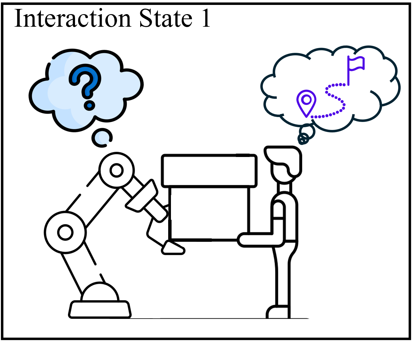
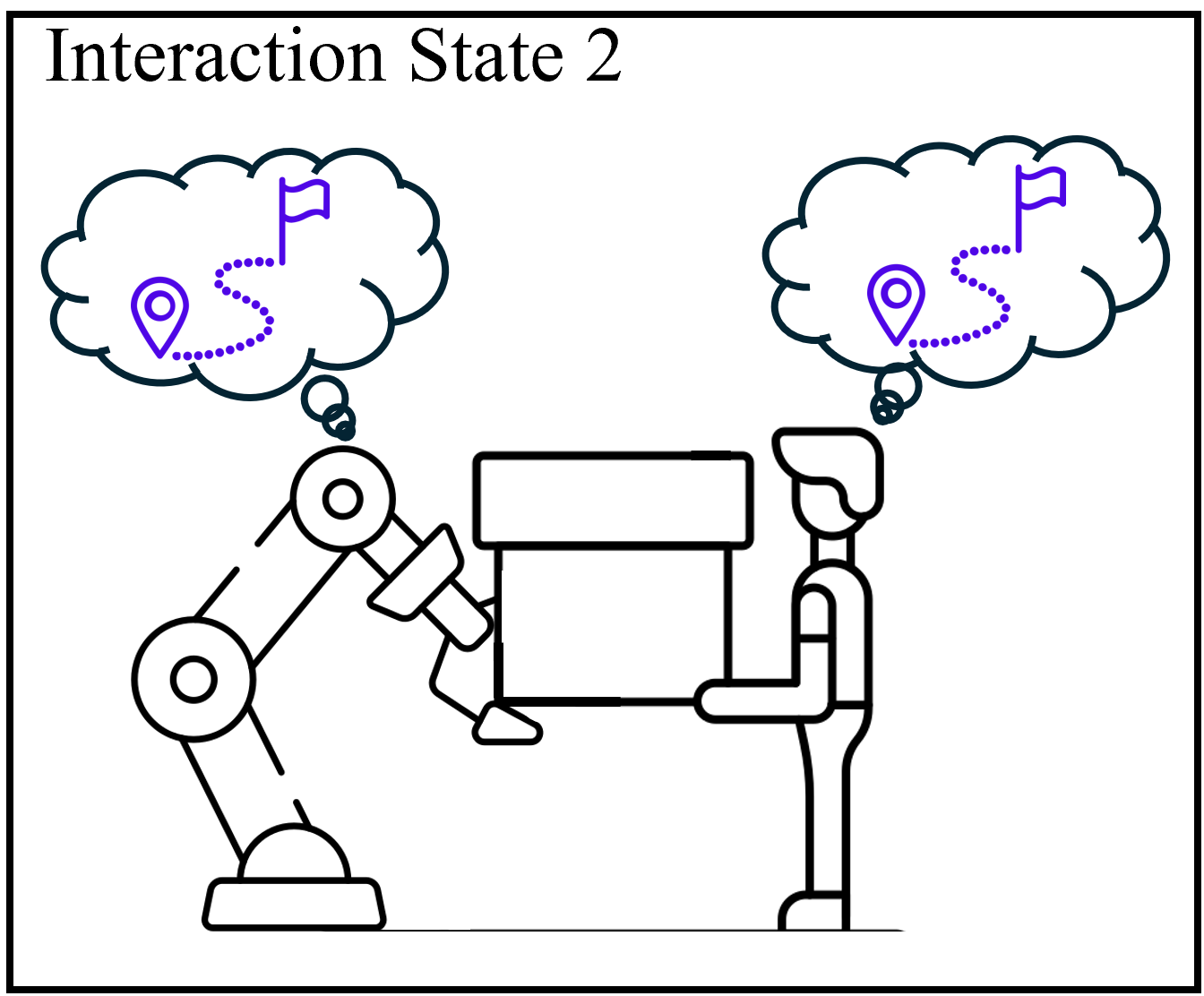
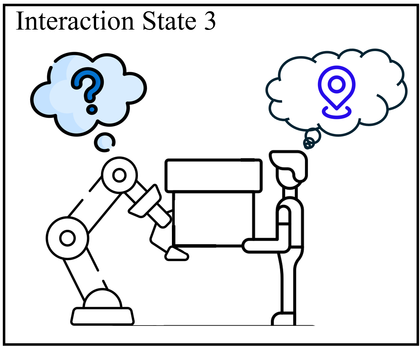
In this paper, we consider co-carrying situations where a human operator and a robot arm grab a single object firmly, which is depicted in Fig. 1. For this collaboration scenario, we assume that the estimated human motion intentions are somehow accessible; however, errors or measurement noises may occasionally be present in these estimations. Therefore, three interaction states of human–robot co-carrying tasks are defined as follows.

•

State 1 (Conflict in Direction): Conflict in direction occurs due to the difference in collaborative transportation trajectory (Fig. 1a). Specifically, the estimated human intention for the robot includes errors.
•

State 2 (Harmonious Movement): As shown in Fig. 1b, the co-carrying trajectory of the robot partner aligns with the human motion intention, thereby generating harmonious human–robot movement.
•

State 3 (Conflict in Parking Location): In Fig. 1c, the human suddenly changes his/her intention to stop at a target location, meanwhile, the robot partner continuously follows the previous co-carrying path that conflicts with the new human intention.

According to the human–robot co-carrying task with the three interaction states, we expect to design a cooperation control framework that satisfies the following features.

(P1)

If the estimated human motion is sufficiently accurate, the robot partner moves the co-carrying object proactively with small human–robot interaction forces. On the contrary, the robot detects conflicts and re-generates the trajectory based on the conflict information.
(P2)

The robot system is strictly passive with respect to the external force–velocity pair when the kinetic energy is higher than the desired one. The kinetic energy of the entire system converges to the predetermined energy level in a finite time interval. Moreover, the power flow from the robot to the human and vice versa can be reduced.
(P3)

In the absence of external forces, the position and velocity of the robot system converge to the human intended position and desired time-varying velocity field, respectively.

II-B Preliminaries

Definition 1

[34] A dynamic system is strictly passive with respect to the pair of input $\mathbf{u}$ and output $\mathbf{y}$ if there is a positive definite storage function $S\left(\mathbf{z}\right)$ and a positive definite dissipative function $D\left(\mathbf{z}\right)$ such that the following relationship holds for all $t\geq 0$ :

S\left(\mathbf{z}\left(t\right)\right)-S\left(\mathbf{z}\left(0\right)\right)\leq\int\limits_{0}^{t}{{{\mathbf{y}}^{\top}}\left(\tau\right)\mathbf{u}\left(\tau\right)d\tau-}\int\limits_{0}^{t}{D\left(\mathbf{z}\left(\tau\right)\right)d\tau},

(1)

in which $\mathbf{z}$ is the state vector.

Lemma 1

[35] The following inequality holds for any real number that satisfies ${{z}_{i}},\,\,i={1,\ldots,n}$ and $0<r<1$ :

\sum\limits_{i=1}^{n}{{{\left|{{z}_{i}}\right|}^{r}}}\geq{{\left(\sum\limits_{i=1}^{n}{\left|{{z}_{i}}\right|}\right)}^{r}}

(2)

Lemma 2

(Cauchy–Schwarz inequality) [36] For arbitrary $\mathbf{A},\,\,\mathbf{B}\in{\mathbb{R}^{n}}$ , the following inequality holds:

{{\left({{\mathbf{A}}^{\top}}\mathbf{B}\right)}^{2}}\leq\left({{\mathbf{A}}^{\top}}\mathbf{A}\right)\left({{\mathbf{B}}^{\top}}\mathbf{B}\right)

(3)

III Proposed Methodology

III-A System Description

The dynamics of a fully actuated $n$ -link robot manipulator is presented as,

\mathbf{M}\left(\mathbf{q}\right)\mathbf{\ddot{q}}+\mathbf{C}\left(\mathbf{q},\mathbf{\dot{q}}\right)\mathbf{\dot{q}}=\boldsymbol{\tau}+{{\boldsymbol{\tau}}_{ext}},

(4)

in which $\mathbf{q}={{\left[\begin{matrix}{{q}_{1}}&{{q}_{2}}&\ldots&{{q}_{n}}\\ \end{matrix}\right]}^{\top}}\in{{\mathbb{R}}^{{n}}}$ is the joint displacement vector, $\mathbf{M}\left(\mathbf{q}\right)$ and $\mathbf{C}\left(\mathbf{q},\mathbf{\dot{q}}\right)\in{{\mathbb{R}}^{{n\times n}}}$ denote the inertia, Coriolis and centrifugal matrices, respectively. $\boldsymbol{\tau}$ and ${{\boldsymbol{\tau}}_{ext}}\in{{\mathbb{R}}^{{n}}}$ are the control torque acting at the actuators and external torque from the interaction with the human operator, correspondingly. To guarantee the passivity of the system, the robot manipulator model in (4) is augmented with a fictitious flywheel state that serves as a fictitious energy storage component. The dynamics of the fictitious flywheel is defined as:

{{m}_{f}}{{\ddot{q}}_{f}}={{\tau}_{f}},

(5)

where ${{m}_{f}}$ and ${{q}_{f}}$ represent the mass and angular position of the flywheel, ${{\tau}_{f}}$ is the control torque exerted on the flywheel. By combining the dynamic model of the robot manipulator in (4) and fictitious flywheel in (5), an augmented system is given as,

{{\mathbf{M}}^{a}}\left({{\mathbf{q}}^{a}}\right){{\mathbf{\ddot{q}}}^{a}}+{{\mathbf{C}}^{a}}\left({{\mathbf{q}}^{a}},{{{\mathbf{\dot{q}}}}^{a}}\right){{\mathbf{\dot{q}}}^{a}}={{\boldsymbol{\tau}}^{a}}+\boldsymbol{\tau}_{ext}^{a},

(6)

in which ${{\mathbf{q}}^{a}}={{\left[\begin{matrix}{{q}_{1}}&{{q}_{2}}&\ldots&\begin{matrix}{{q}_{n}}&{{q}_{f}}\\ \end{matrix}\\ \end{matrix}\right]}^{\top}}\in{{\mathbb{R}}^{n+1}}$ represents the joint angle vector, ${{\boldsymbol{\tau}}^{a}}={{\left[\begin{matrix}{{\boldsymbol{\tau}}^{\top}}&{{\tau}_{f}}\\ \end{matrix}\right]}^{\top}}$ and $\boldsymbol{\tau}_{ext}^{a}={{\left[\begin{matrix}\boldsymbol{\tau}_{ext}^{\top}&0\\ \end{matrix}\right]}^{\top}}$ are the augmented control input and external force vector, respectively. ${{\mathbf{M}}^{a}}\left({{\mathbf{q}}^{a}}\right)\,=\left[\begin{matrix}\mathbf{M}\left(\mathbf{q}\right)&{{\mathbf{0}}_{n\times 1}}\\ {{\mathbf{0}}_{1\times n}}&{{m}_{f}}\\ \end{matrix}\right]$ and ${{\mathbf{C}}^{a}}\left({{\mathbf{q}}^{a}},{{{\mathbf{\dot{q}}}}^{a}}\right)=\left[\begin{matrix}\mathbf{C}\left(\mathbf{q},\mathbf{\dot{q}}\right)&{{\mathbf{0}}_{n\times 1}}\\ {{\mathbf{0}}_{1\times n}}&0\\ \end{matrix}\right]$ are the augmented inertia matrix and Coriolis matrix, correspondingly. ${{\mathbf{M}}^{a}}$ denotes a positive-definite symmetric matrix and $\left({{{\mathbf{\dot{M}}}}^{a}}\left({{\mathbf{q}}^{a}}\right)-2{{\mathbf{C}}^{a}}\left({{\mathbf{q}}^{a}},{{{\mathbf{\dot{q}}}}^{a}}\right)\right)$ is a skew-symmetric matrix.

III-B Cooperation Control Framework Design

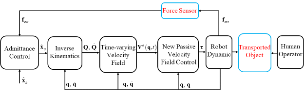
In this section, a cooperation control framework with two parts is designed for collaboratively transporting a rigid object as shown in Fig. 2, including a time-varying Velocity Field Generation part and a PVFC part.

Regarding the first part, an Admittance Control with mass–damper (MD) features is presented to modify the desired co-carrying trajectory for the robot partner according to the conflict detection through the force sensor signal ${{\mathbf{f}}_{ext}}$ .

{{\mathbf{M}}_{d}}\left({{{\mathbf{\ddot{x}}}}_{a}}-{{{\mathbf{\ddot{\hat{x}}}}}_{h}}\right)+{{\mathbf{D}}_{d}}\left({{{\mathbf{\dot{x}}}}_{a}}-{{{\mathbf{\dot{\hat{x}}}}}_{h}}\right)={{\mathbf{f}}_{ext}},

(7)

where ${{\mathbf{M}}_{d}}$ and ${{\mathbf{D}}_{d}}$ are inertia and damping matrices, respectively. ${{\mathbf{x}}_{a}}$ represents the desired trajectory obtained from (7) and ${{{\mathbf{\hat{x}}}}_{h}}$ is the estimated human motion intention. ${{\mathbf{f}}_{ext}}$ denotes the external force that is applied by the human. Based on (7), the characteristics of the proposed Admittance Control are stated as follows:

•

In the case of estimating human intention precisely, the human–robot interaction force $\left({{\mathbf{f}}_{ext}}\right)$ is very small or ideally zero; therefore, the desired trajectory $\left({{\mathbf{x}}_{a}}\right)$ closely aligns with the estimated human intention $\left({{{\mathbf{\hat{x}}}}_{h}}\right)$ ; and
•

the desired co-carrying trajectory $\left({{\mathbf{x}}_{a}}\right)$ is modified according to the interaction force $\left({{\mathbf{f}}_{ext}}\right)$ on the contrary.

By utilizing the Admittance Control output $\left({{{\mathbf{\dot{x}}}}_{a}}\right)$ , the time-varying Velocity Field $\left(\mathbf{V}\left(\mathbf{q},t\right)\right)$ of the robot manipulator in (4) is created as a sliding surface.

\left\{\begin{aligned} &\mathbf{\dot{Q}}\left(t\right)={{\mathbf{J}}^{+}}\left(\mathbf{q}\right){{{\mathbf{\dot{x}}}}_{a}}\left(t\right)\\ &\mathbf{V}\left(\mathbf{q},t\right)=\mathbf{\dot{Q}}\left(t\right)-{{\mathbf{K}}_{1}}\left(\mathbf{q}\left(t\right)-\mathbf{Q}\left(t\right)\right),\\ \end{aligned}\right.

(8)

in which ${{\mathbf{J}}^{+}}\left(\mathbf{q}\right)={{\left({{\mathbf{J}}^{\top}}\left(\mathbf{q}\right)\mathbf{J}\left(\mathbf{q}\right)\right)}^{-1}}{{\mathbf{J}}^{\top}}\left(\mathbf{q}\right)$ with the Jacobian matrix $\mathbf{J}\left(\mathbf{q}\right)$ and $\mathbf{Q}\left(t\right)$ is the reference angular position. ${{\mathbf{K}}_{1}}$ denotes the positive-definite control parameter matrix. Additionally, the desired Velocity Field ${{V}_{f}}\left(\mathbf{q},t\right)$ of the fictitious flywheel is calculated as:

{{V}_{f}}\left(\mathbf{q},t\right)=\sqrt{\frac{2}{{{m}_{f}}}\left({{E}^{a}}-\frac{1}{2}{{\mathbf{V}}^{\top}}\left(\mathbf{q},t\right)\mathbf{M}\left(\mathbf{q}\right)\mathbf{V}\left(\mathbf{q},t\right)\right)}

(9)

Note that ${{E}^{a}}$ denotes a sufficiently large positive constant, which ensures the formulation under the square root is positive. As a result, the desired time-varying Velocity Field $\left({{\mathbf{V}}^{a}}\left({{\mathbf{q}}},t\right)={{\left[\begin{matrix}{{\mathbf{V}}^{\top}}\left(\mathbf{q},t\right)&{{V}_{f}}\left(\mathbf{q},t\right)\\ \end{matrix}\right]}^{\top}}\right)$ of the augmented system in (6), which satisfies consistency and the following conservation of kinetic energy principle, is defined.

		$\displaystyle{{k}^{a}}\left({{\mathbf{q}}^{a}},\,\,{{\mathbf{V}}^{a}}\left(\mathbf{q},t\right)\right)=\frac{1}{2}{{\mathbf{V}}^{a}}^{\top}\left(\mathbf{q},t\right){{\mathbf{M}}^{a}}\left({{\mathbf{q}}^{a}}\right){{\mathbf{V}}^{a}}\left(\mathbf{q},t\right)$		(10)
		$\displaystyle\,\,\,\,\,\,\,\,\,\,\,\,\,\,\,\,=\frac{1}{2}{{\mathbf{V}}^{\top}}\left(\mathbf{q},t\right)\mathbf{M}\left(\mathbf{q}\right)\mathbf{V}\left(\mathbf{q},t\right)+\frac{1}{2}{{m}_{f}}V_{f}^{2}\left(\mathbf{q},t\right)$
		$\displaystyle\,\,\,\,\,\,\,\,\,\,\,\,\,\,\,\,={{E}^{a}}>0,$

in which ${{k}^{a}}\left({{\mathbf{q}}^{a}},\,\,{{\mathbf{V}}^{a}}\left(\mathbf{q},t\right)\right)$ is the kinetic energy of the desired Velocity Field. Thereafter, the actual kinetic energy $\left({{k}^{a}}\left({{\mathbf{q}}^{a}},\,\,{{{\mathbf{\dot{q}}}}^{a}}\right)\right)$ of the augmented system is computed as,

		$\displaystyle{{k}^{a}}\left({{\mathbf{q}}^{a}},\,\,{{\mathbf{\dot{q}}}^{a}}\right)=\frac{1}{2}{{\mathbf{\dot{q}}}^{a\top}}{{\mathbf{M}}^{a}}\left({{\mathbf{q}}^{a}}\right){{{\mathbf{\dot{q}}}}^{a}}$		(11)
		$\displaystyle\,\,\,\,\,\,\,\,\,\,\,\,\,\,\,\,\,\,\,\,\,\,\,\,\,\,\,\,\,\,=\frac{1}{2}{{{\mathbf{\dot{q}}}}^{\top}}\mathbf{M}\left(\mathbf{q}\right)\mathbf{\dot{q}}+\frac{1}{2}{{m}_{f}}\dot{q}_{f}^{2},$		(11)

Concerning the second part of the cooperation control framework, a new PVFC is designed to guarantee the passivity of the closed-loop system. The approach in [33] is inherited in order to control the power flow into the human operator, such that it enhances the safety of the human and co-transported object. Furthermore, we newly propose a fractional exponent control term to compensate for the kinetic energy of the augmented system in a finite time interval. Based on (7)–(11), the new PVFC with a fractional exponent energy compensation control term is developed for the ${{\boldsymbol{\tau}}^{a}}\left({{\mathbf{q}}^{a}},\,\,{{{\mathbf{\dot{q}}}}^{a}},t\right)$ of the augmented system in (6) as,

		$\displaystyle{{\boldsymbol{\tau}}^{a}}\left({{\mathbf{q}}^{a}},\,\,{{{\mathbf{\dot{q}}}}^{a}},t\right)=\left[\mathbf{G}\left({{\mathbf{q}}^{a}},\,\,{{{\mathbf{\dot{q}}}}^{a}},t\right)+\mathbf{R}\left({{\mathbf{q}}^{a}},\,\,{{{\mathbf{\dot{q}}}}^{a}},t\right)\right]{{{\mathbf{\dot{q}}}}^{a}}$		(12)
		$\displaystyle\,\,\,\,\,\,\,\,\,\,\,\,\,\,\,\,\,\,\,\,\,\,\,\,\,\,\,\,\,\,\,\,\,\,\,\,\,\,\,\,\,\,\,\,\,\,\,\,\,\,\,\,\,\,\,\,\,\,\,\,\,\,\,\,\,\,\,\,\,\,\,\,-\mathbf{S}\left({{\mathbf{q}}^{a}},\,\,{{{\mathbf{\dot{q}}}}^{a}}\right){{\left[{{{\mathbf{\dot{q}}}}^{a}}\right]}^{\frac{{{r}_{1}}}{{{r}_{2}}}}},$		(12)

in which $\mathbf{S}\left({{\mathbf{q}}^{a}},\,\,{{{\mathbf{\dot{q}}}}^{a}}\right){{\left[{{{\mathbf{\dot{q}}}}^{a}}\right]}^{\frac{{{r}_{1}}}{{{r}_{2}}}}}$ is utilized to compensate for the kinetic energy of the augmented system within a finite time interval. Two skew-symmetric matrices $\mathbf{G}\left({{\mathbf{q}}^{a}},\,\,{{{\mathbf{\dot{q}}}}^{a}},t\right)$ , $\mathbf{R}\left({{\mathbf{q}}^{a}},\,\,{{{\mathbf{\dot{q}}}}^{a}},t\right)$ , and a diagonal matrix $\mathbf{S}\left({{\mathbf{q}}^{a}},\,\,{{{\mathbf{\dot{q}}}}^{a}}\right)$ are designed in the following formulation.

\left\{\begin{aligned} &\mathbf{G}\left({{\mathbf{q}}^{a}},\,\,{{{\mathbf{\dot{q}}}}^{a}},t\right):=\frac{1}{2{{E}^{a}}}\left(\mathbf{w}{{\mathbf{P}}^{\top}}-\mathbf{P}{{\mathbf{w}}^{\top}}\right)\\ &\mathbf{R}\left({{\mathbf{q}}^{a}},\,\,{{{\mathbf{\dot{q}}}}^{a}},t\right):=\kappa\left(\mathbf{P}{{\mathbf{p}}^{\top}}-\mathbf{p}{{\mathbf{P}}^{\top}}\right)\\ &\mathbf{S}\left({{\mathbf{q}}^{a}},\,\,{{{\mathbf{\dot{q}}}}^{a}}\right):=s\left({{k}^{a}}\left({{\mathbf{q}}^{a}},\,\,{{{\mathbf{\dot{q}}}}^{a}}\right)-k_{d}^{a}\right){{\mathbf{K}}_{2}},\\ \end{aligned}\right.

(13)

where $\kappa$ is control parameters and $k_{d}^{a}$ is the desired kinetic energy level of the augmented system. Furthermore, to avoid clutter, $\mathbf{w}=\mathbf{w}\left({{\mathbf{q}}^{a}},\,\,{{{\mathbf{\dot{q}}}}^{a}},t\right)$ , $\mathbf{P}=\mathbf{P}\left({{\mathbf{q}}^{a}},t\right)$ , and $\mathbf{p}=\mathbf{p}\left({{\mathbf{q}}^{a}},\,\,{{{\mathbf{\dot{q}}}}^{a}}\right)$ are utilized in the paper. The inverse dynamics with the desired time-varying Velocity Field $\left(\mathbf{w}\right)$ , desired momentum $\left(\mathbf{P}\right)$ , and actual momentum $\left(\mathbf{p}\right)$ of the augmented system in (6), as well as the diagonal positive-definite matrix $\left({{\mathbf{K}}_{2}}\right)$ are defined as:

\left\{\begin{aligned} &\mathbf{w}={{\mathbf{M}}^{a}}\left({{\mathbf{q}}^{a}}\right){{{\mathbf{\dot{V}}}}^{a}}\left(\mathbf{q},t\right)+{{\mathbf{C}}^{a}}\left({{\mathbf{q}}^{a}},\,\,{{{\mathbf{\dot{q}}}}^{a}}\right){{\mathbf{V}}^{a}}\left(\mathbf{q},t\right)\\ &\mathbf{P}={{\mathbf{M}}^{a}}\left({{\mathbf{q}}^{a}}\right){{\mathbf{V}}^{a}}\left(\mathbf{q},t\right)\\ &\mathbf{p}={{\mathbf{M}}^{a}}\left({{\mathbf{q}}^{a}}\right){{{\mathbf{\dot{q}}}}^{a}}\\ &{{\mathbf{K}}_{2}}=\text{diag}\left({{k}_{21}},{{k}_{22}},\ldots,{{k}_{2n}},{{k}_{2f}}\right),\\ \end{aligned}\right.

(14)

where the $i$ -th term of the differential of the time-varying Velocity Field is computed as follows,

\dot{V}_{i}^{a}\left(\mathbf{q},t\right)=\sum\limits_{j=1}^{n+1}{\frac{\partial V_{i}^{a}\left(\mathbf{q},t\right)}{\partial q_{j}^{a}}\dot{q}_{j}^{a}}+\frac{\partial V_{i}^{a}\left(\mathbf{q},t\right)}{\partial t}.

(15)

Additionally, the fractional exponent of the augmented velocity in (12) is defined by:

		$\displaystyle{{\left[{{{\mathbf{\dot{q}}}}^{a}}\right]}^{\frac{{{r}_{1}}}{{{r}_{2}}}}}=\left[\begin{matrix}{\mathop{\rm sgn}}\left({{{\dot{q}}}_{1}}\right){{\left\|{{{\dot{q}}}_{1}}\right\|}^{\frac{{{r}_{1}}}{{{r}_{2}}}}}&{\mathop{\rm sgn}}\left({{{\dot{q}}}_{2}}\right){{\left\|{{{\dot{q}}}_{2}}\right\|}^{\frac{{{r}_{1}}}{{{r}_{2}}}}}&\ldots\\ \end{matrix}\right.$		(16)
		$\displaystyle\,\,\,\,\,\,\,\,\,\,\,\,\,\,\,\,\,\,\,\,\,\,\,\,\,\,\,\,\,\,\,\,\,\,\,\,\,\,\,\,\,{{\left.\begin{matrix}{\mathop{\rm sgn}}\left({{{\dot{q}}}_{n}}\right){{\left\|{{{\dot{q}}}_{n}}\right\|}^{\frac{{{r}_{1}}}{{{r}_{2}}}}}&{\mathop{\rm sgn}}\left({{{\dot{q}}}_{f}}\right){{\left\|{{{\dot{q}}}_{f}}\right\|}^{\frac{{{r}_{1}}}{{{r}_{2}}}}}\\ \end{matrix}\right]}^{T}},$		(16)

with ${{r}_{1}},\,{{r}_{2}}$ $\left({{r}_{1}}<{{r}_{2}}\right)$ are positive odd integers. The smooth saturation function in (13) is designed to compensate for the kinetic energy of the augmented system.

s\left(e\right)=\left\{\begin{aligned} &{{\eta}_{\min}}\,\,\,\,\,\,\,\,\,\,\,\,\,\,\,\,\,\,\,\,\,\,\,\,\,\,\,\,\,\,\,\,\,\,\,\,\,\,\,\,\,\,\,\,\,\,\,\,\,\,\,\,\,\,\,\,\,\,\,\,\,\,\,\,\,e<{{\delta}_{1}}\\ &\frac{{{\eta}_{\min}}}{2}\left(1-\cos\left(\frac{\pi}{{{\delta}_{1}}}e\right)\right)\,\,\,\,\,\,\,\,\,\,{{\delta}_{1}}\leq e<0\,\\ &0\,\,\,\,\,\,\,\,\,\,\,\,\,\,\,\,\,\,\,\,\,\,\,\,\,\,\,\,\,\,\,\,\,\,\,\,\,\,\,\,\,\,\,\,\,\,\,\,\,\,\,\,\,\,\,\,\,\,\,\,\,\,\,\,\,\,\,\,\,\,\,\,\,\,\,\,e=0\\ &\frac{{{\eta}_{\max}}}{2}\left(1-\cos\left(\frac{\pi}{{{\delta}_{2}}}e\right)\right)\,\,\,\,\,\,\,\,\,0<e\leq{{\delta}_{2}}\,\\ &{{\eta}_{\max}}\,\,\,\,\,\,\,\,\,\,\,\,\,\,\,\,\,\,\,\,\,\,\,\,\,\,\,\,\,\,\,\,\,\,\,\,\,\,\,\,\,\,\,\,\,\,\,\,\,\,\,\,\,\,\,\,\,\,\,\,\,\,\,\,\,\,e>{{\delta}_{2}}\\ \end{aligned}\right.

(17)

where $e={{k}^{a}}\left({{\mathbf{q}}^{a}},\,\,{{{\mathbf{\dot{q}}}}^{a}}\right)-k_{d}^{a}$ and ${{\eta}_{\min}}<0$ , ${{\eta}_{\max}}>0$ , ${{\delta}_{2}}>0$ , ${{\delta}_{1}}<0$ are constants.

III-C Main Results

Theorem 1

(Passivity) Leveraging the action of control commands in (12) for the augmented system in (6), the kinetic energy of the system in (11) satisfies:

		$\displaystyle\frac{d}{dt}{{k}^{a}}\left({{\mathbf{q}}^{a}},\,\,{{{\mathbf{\dot{q}}}}^{a}}\right)=\boldsymbol{\tau}_{ext}^{a\top}{{{\mathbf{\dot{q}}}}^{a}}$		(18)
		$\displaystyle\,\,\,\,\,\,\,\,\,\,\,\,\,\,-s\left({{k}^{a}}\left({{\mathbf{q}}^{a}},\,\,{{{\mathbf{\dot{q}}}}^{a}}\right)-k_{d}^{a}\right){{{\mathbf{\dot{q}}}}^{a\top}}{{\mathbf{K}}_{2}}{{\left[{{{\mathbf{\dot{q}}}}^{a}}\right]}^{\frac{{{r}_{1}}}{{{r}_{2}}}}},$		(18)

in which ${{r}_{1}},\,{{r}_{2}}$ $\left({{r}_{1}}<{{r}_{2}}\right)$ are positive odd integers and ${{\mathbf{K}}_{2}}$ is a positive-definite matrix. According to Definition 1, the closed-loop system is strictly passive with respect to the pair of the velocity output $\left({{{\mathbf{\dot{q}}}}^{a}}\right)$ and external force input $\left(\boldsymbol{\tau}_{ext}^{a}\right)$ under the condition ${{k}^{a}}\left({{\mathbf{q}}^{a}},\,\,{{{\mathbf{\dot{q}}}}^{a}}\right)-k_{d}^{a}\geq 0$ .

Theorem 2

(Convergence time of kinetic energy) Under the new PVFC in (12) with positive odd integers $\left({{r}_{1}},\,{{r}_{2}}\,\,\left({{r}_{1}}<{{r}_{2}}\right)\right)$ and positive-definite matrix $\left({{\mathbf{K}}_{2}}\right)$ , the kinetic energy of the augmented system ${{k}^{a}}\left({{\mathbf{q}}^{a}},{{{\mathbf{\dot{q}}}}^{a}}\right)$ converges to the desired one $k_{d}^{a}$ within a finite time interval in the absence of external disturbance $\left(\boldsymbol{\tau}_{ext}^{a}=0\right)$ . The settling time of the system $\left(T\right)$ is bounded by,

T\leq\max\left\{{{T}_{1}},{{T}_{2}}\right\},

(19)

where $T_{1}$ and $T_{2}$ are correspondingly the convergence times with ${{k}^{a}}\left({{\mathbf{q}}^{a}},{{{\mathbf{\dot{q}}}}^{a}}\right)\geq k_{d}^{a}$ and ${{k}^{a}}\left({{\mathbf{q}}^{a}},{{{\mathbf{\dot{q}}}}^{a}}\right)<k_{d}^{a}$ , which are specifically calculated in the next subsection.

Theorem 3

(Stability) By applying the control inputs of the new time-varying PVFC in (8) and (12) and designing the positive-definite control parameters $\left({{\mathbf{K}}_{2}},\,\,\kappa\right)$ , the solutions

\left\{\begin{aligned} &{{\mathbf{e}}_{\mathbf{q}}}=\mathbf{q}\left(t\right)-\mathbf{Q}\left(t\right)=\mathbf{0}\\ &{{\mathbf{e}}_{\mathbf{v}}}={{{\mathbf{\dot{q}}}}^{a}}\left(t\right)-\alpha\left(t\right){{\mathbf{V}}^{a}}\left({{\mathbf{q}}^{a}}\left(t\right),t\right)=\mathbf{0}\\ \end{aligned}\right.

(20)

to the augmented system in (6) is Lyapunov stable in the absence of external disturbance $\left(\boldsymbol{\tau}_{ext}^{a}=0\right)$ . The $\alpha\left(t\right)$ term is defined such that:

\alpha\left(t\right)=\sqrt{\frac{{{k}^{a}}\left({{\mathbf{q}}^{a}}\left(t\right),{{{\mathbf{\dot{q}}}}^{a}}\left(t\right)\right)}{{{E}^{a}}}}.

(21)

Lemma 3

(Power flow) When the external force $\left(\boldsymbol{\tau}_{ext}^{a}\right)$ is applied by the human operator, the power flow into the human and robot is calculated by the augmented system in (6) and the control command in (12) as follows:

{{P}_{r2h}}\,\,=-s\left({{k}^{a}}\left(\mathbf{q},{{\mathbf{q}}^{a}}\right)-k_{d}^{a}\right){{\mathbf{\dot{q}}}^{aT}}{{\mathbf{K}}_{2}}{{\left[{{{\mathbf{\dot{q}}}}^{a}}\right]}^{\frac{{{r}_{1}}}{{{r}_{2}}}}}-{{\dot{k}}^{a}},

(22)

in which ${{P}_{r2h}}\,>0$ with ${{k}^{a}}\left(\mathbf{q},{{\mathbf{q}}^{a}}\right)<k_{d}^{a}$ is the power flow from the robot to the human; meanwhile, ${{P}_{r2h}}\,<0$ with ${{k}^{a}}\left(\mathbf{q},{{\mathbf{q}}^{a}}\right)\geq k_{d}^{a}\,$ denotes the power flowing from the human to the robot. By adjusting the control parameters $\left({{\mathbf{K}}_{2}},\,\,{{\eta}_{\max}},\,\,\,{{\eta}_{\min}},\,\,{{\delta}_{1}},\,\,{{\delta}_{2}}\right)$ in (13) and (17), we can reduce the power flow into the human operator, robot partner, and co-transported object.

III-D Proof

Proof of Theorem 1

Differentiating the kinetic energy in (11) and utilizing the augmented system in (6), yields:

		$\displaystyle\frac{d}{dt}{{k}^{a}}\left({{\mathbf{q}}^{a}},\,\,{{{\mathbf{\dot{q}}}}^{a}}\right)$		(23)
		$\displaystyle={{{\mathbf{\dot{q}}}}^{a\top}}{{\mathbf{M}}^{a}}{{{\mathbf{\ddot{q}}}}^{a}}+\frac{1}{2}{{{\mathbf{\dot{q}}}}^{a\top}}{{{\mathbf{\dot{M}}}}^{a}}{{{\mathbf{\dot{q}}}}^{a}}$
		$\displaystyle=\frac{1}{2}{{{\mathbf{\dot{q}}}}^{a\top}}{{{\mathbf{\dot{M}}}}^{a}}{{{\mathbf{\dot{q}}}}^{a}}+{{{\mathbf{\dot{q}}}}^{a\top}}\left({{\boldsymbol{\tau}}^{a}}+\boldsymbol{\tau}_{ext}^{a}-{{\mathbf{C}}^{a}}\left({{\mathbf{q}}^{a}},{{{\mathbf{\dot{q}}}}^{a}}\right){{{\mathbf{\dot{q}}}}^{a}}\right).$

Substituting the new time-varying PVFC in (12) into (23), we obtain,

		$\displaystyle\frac{d}{dt}{{k}^{a}}\left({{\mathbf{q}}^{a}},\,\,{{{\mathbf{\dot{q}}}}^{a}}\right)=\frac{1}{2}{{{\mathbf{\dot{q}}}}^{a\top}}\left({{{\mathbf{\dot{M}}}}^{a}}-2{{\mathbf{C}}^{a}}\left({{\mathbf{q}}^{a}},{{{\mathbf{\dot{q}}}}^{a}}\right)\right){{{\mathbf{\dot{q}}}}^{a}}$		(24)
		$\displaystyle\,\,\,\,\,\,\,\,\,\,\,\,\,\,\,\,\,\,+{{{\mathbf{\dot{q}}}}^{a\top}}\mathbf{R}\left({{\mathbf{q}}^{a}},\,\,{{{\mathbf{\dot{q}}}}^{a}},t\right){{{\mathbf{\dot{q}}}}^{a}}+{{{\mathbf{\dot{q}}}}^{a\top}}\mathbf{G}\left({{\mathbf{q}}^{a}},\,\,{{{\mathbf{\dot{q}}}}^{a}},t\right){{{\mathbf{\dot{q}}}}^{a}}$
		$\displaystyle\,\,\,\,\,\,\,\,\,\,\,\,\,\,\,\,\,\,+{{{\mathbf{\dot{q}}}}^{a\top}}\boldsymbol{\tau}_{ext}^{a}-{{{\mathbf{\dot{q}}}}^{a\top}}\mathbf{S}\left({{\mathbf{q}}^{a}},\,\,{{{\mathbf{\dot{q}}}}^{a}}\right){{\left[{{{\mathbf{\dot{q}}}}^{a}}\right]}^{\frac{{{r}_{1}}}{{{r}_{2}}}}},$

in which ${{\mathbf{\dot{M}}}^{a}}-2{{\mathbf{C}}^{a}}\left({{\mathbf{q}}^{a}},{{{\mathbf{\dot{q}}}}^{a}}\right),\,\,\mathbf{G}\left({{\mathbf{q}}^{a}},{{{\mathbf{\dot{q}}}}^{a}},t\right),\,\,\mathbf{R}\left({{\mathbf{q}}^{a}},{{{\mathbf{\dot{q}}}}^{a}},t\right)$ are skew-symmetric matrices; therefore, equation (24) becomes:

		$\displaystyle\frac{d}{dt}{{k}^{a}}\left({{\mathbf{q}}^{a}},\,\,{{{\mathbf{\dot{q}}}}^{a}}\right)$		(25)
		$\displaystyle={{{\mathbf{\dot{q}}}}^{a\top}}\boldsymbol{\tau}_{ext}^{a}-{{{\mathbf{\dot{q}}}}^{a\top}}\mathbf{S}\left({{\mathbf{q}}^{a}},\,\,{{{\mathbf{\dot{q}}}}^{a}}\right){{\left[{{{\mathbf{\dot{q}}}}^{a}}\right]}^{\frac{{{r}_{1}}}{{{r}_{2}}}}}$
		$\displaystyle=\boldsymbol{\tau}_{ext}^{a\top}{{{\mathbf{\dot{q}}}}^{a}}-s\left({{k}^{a}}\left({{\mathbf{q}}^{a}},\,\,{{{\mathbf{\dot{q}}}}^{a}}\right)-k_{d}^{a}\right){{{\mathbf{\dot{q}}}}^{a\top}}{{\mathbf{K}}_{2}}{{\left[{{{\mathbf{\dot{q}}}}^{a}}\right]}^{\frac{{{r}_{1}}}{{{r}_{2}}}}}.$

By integrating both sides of (25) over the time interval $\left[0,t\right]$ , we have:

		$\displaystyle\int\limits_{0}^{t}{{{{\mathbf{\dot{q}}}}^{a\top}}\boldsymbol{\tau}_{ext}^{a}d\tau}={{k}^{a}}\left({{\mathbf{q}}^{a}}\left(t\right),{{{\mathbf{\dot{q}}}}^{a}}\left(t\right)\right)-{{k}^{a}}\left({{\mathbf{q}}^{a}}\left(0\right),{{{\mathbf{\dot{q}}}}^{a}}\left(0\right)\right)$		(26)
		$\displaystyle\,\,\,\,\,\,\,\,\,\,\,\,\,\,\,\,\,\,\,\,\,\,\,\,\,\,\,\,\,\,\,\,\,\,\,\,\,\,\,\,\,\,\,\,\,\,\,\,\,\,\,\,\,\,\,\,\,\,\,\,\,\,\,\,\,\,\,+\int\limits_{0}^{t}{{{{\mathbf{\dot{q}}}}^{a\top}}\mathbf{S}\left({{\mathbf{q}}^{a}},{{{\mathbf{\dot{q}}}}^{a}}\right){{\left[{{{\mathbf{\dot{q}}}}^{a}}\right]}^{\frac{{{r}_{1}}}{{{r}_{2}}}}}}d\tau.$		(26)

Obviously, if ${{r}_{1}},\,{{r}_{2}}$ $\left({{r}_{1}}<{{r}_{2}}\right)$ are positive odd intergers and ${{\mathbf{K}}_{2}}$ denotes positive-definite matrix, ${{k}^{a}}\left({{\mathbf{q}}^{a}},\,\,{{{\mathbf{\dot{q}}}}^{a}}\right)>0$ and $\int\limits_{0}^{t}{{{{\mathbf{\dot{q}}}}^{a\top}}\mathbf{S}\left({{\mathbf{q}}^{a}},\,\,{{{\mathbf{\dot{q}}}}^{a}}\right){{\left[{{{\mathbf{\dot{q}}}}^{a}}\right]}^{\frac{{{r}_{1}}}{{{r}_{2}}}}}}d\tau>0$ under ${{k}^{a}}\left({{\mathbf{q}}^{a}},{{{\mathbf{\dot{q}}}}^{a}}\right)-k_{d}^{a}\geq 0$ . Therefore, the closed-loop system is strictly passive when the kinetic energy exceeds the predetermined level.

Proof of Theorem 2

According to Lyapunov’s direct method in [37, 38], a Lyapunov function is selected for examining the convergence of the kinetic energy as follows:

{{V}_{1}}\left({{\mathbf{q}}^{a}},\,\,{{{\mathbf{\dot{q}}}}^{a}}\right)=\frac{1}{2}{{\left({{k}^{a}}\left({{\mathbf{q}}^{a}},{{{\mathbf{\dot{q}}}}^{a}}\right)-k_{d}^{a}\right)}^{2}}.

(27)

Taking the derivative of (27) with respect to time and combining it with the kinetic energy in (11), we have:

		$\displaystyle{{{\dot{V}}}_{1}}\left({{\mathbf{q}}^{a}},\,\,{{{\mathbf{\dot{q}}}}^{a}}\right)$		(28)
		$\displaystyle=\left({{k}^{a}}\left({{\mathbf{q}}^{a}},{{{\mathbf{\dot{q}}}}^{a}}\right)-k_{d}^{a}\right)\left({{{\dot{k}}}^{a}}\left({{\mathbf{q}}^{a}},{{{\mathbf{\dot{q}}}}^{a}}\right)-\dot{k}_{d}^{a}\right)$
		$\displaystyle=\left({{k}^{a}}\left({{\mathbf{q}}^{a}},{{{\mathbf{\dot{q}}}}^{a}}\right)-k_{d}^{a}\right)\left({{{\mathbf{\dot{q}}}}^{a\top}}{{\mathbf{M}}^{a}}{{{\mathbf{\ddot{q}}}}^{a}}+\frac{1}{2}{{{\mathbf{\dot{q}}}}^{a\top}}{{{\mathbf{\dot{M}}}}^{a}}{{{\mathbf{\dot{q}}}}^{a}}\right).$

Substituting the augmented system (6) into (28), yields:

{{\dot{V}}_{1}}=\left({{k}^{a}}\left({{\mathbf{q}}^{a}},{{{\mathbf{\dot{q}}}}^{a}}\right)-k_{d}^{a}\right)\left(\begin{aligned} &\,{{{\mathbf{\dot{q}}}}^{a\top}}\left({{\boldsymbol{\tau}}^{a}}+\boldsymbol{\tau}_{ext}^{a}-{{\mathbf{C}}^{a}}{{{\mathbf{\dot{q}}}}^{a}}\right)\\ &\,\,\,\,\,\,\,\,\,\,\,\,\,\,\,\,\,\,\,\,\,+\frac{1}{2}{{{\mathbf{\dot{q}}}}^{a\top}}{{{\mathbf{\dot{M}}}}^{a}}{{{\mathbf{\dot{q}}}}^{a}}\\ \end{aligned}\right)

(29)

Considering $\boldsymbol{\tau}_{ext}^{a}=\mathbf{0}$ and adopting the time-varying PVFC in (12), we obtain,

{{\dot{V}}_{1}}=\left({{k}^{a}}\left({{\mathbf{q}}^{a}},{{{\mathbf{\dot{q}}}}^{a}}\right)-k_{d}^{a}\right)\left(\begin{aligned} &\frac{1}{2}{{{\mathbf{\dot{q}}}}^{a\top}}\left({{{\mathbf{\dot{M}}}}^{a}}-2{{\mathbf{C}}^{a}}\right){{{\mathbf{\dot{q}}}}^{a}}\\ &+{{{\mathbf{\dot{q}}}}^{a\top}}\mathbf{G}\left({{\mathbf{q}}^{a}},\,\,{{{\mathbf{\dot{q}}}}^{a}},t\right){{{\mathbf{\dot{q}}}}^{a}}\\ &+{{{\mathbf{\dot{q}}}}^{a\top}}\mathbf{R}\left({{\mathbf{q}}^{a}},\,\,{{{\mathbf{\dot{q}}}}^{a}},t\right){{{\mathbf{\dot{q}}}}^{a}}\\ &-{{{\mathbf{\dot{q}}}}^{a\top}}\mathbf{S}\left({{\mathbf{q}}^{a}},\,\,{{{\mathbf{\dot{q}}}}^{a}}\right){{\left[{{{\mathbf{\dot{q}}}}^{a}}\right]}^{\frac{{{r}_{1}}}{{{r}_{2}}}}}\\ \end{aligned}\right)

(30)

It is straightforward to derive the following formulation using the properties of skew-symmetric matrices.

		$\displaystyle{{{\dot{V}}}_{1}}=-\left({{k}^{a}}\left({{\mathbf{q}}^{a}},{{{\mathbf{\dot{q}}}}^{a}}\right)-k_{d}^{a}\right)\left({{{\mathbf{\dot{q}}}}^{a\top}}\mathbf{S}\left({{\mathbf{q}}^{a}},\,\,{{{\mathbf{\dot{q}}}}^{a}}\right){{\left[{{{\mathbf{\dot{q}}}}^{a}}\right]}^{\frac{{{r}_{1}}}{{{r}_{2}}}}}\right)$		(31)
		$\displaystyle\,\,\,\,\,\,\,=-\left({{k}^{a}}\left({{\mathbf{q}}^{a}},{{{\mathbf{\dot{q}}}}^{a}}\right)-k_{d}^{a}\right)s\left(e\right)\left({{{\mathbf{\dot{q}}}}^{a\top}}{{\mathbf{K}}_{2}}{{\left[{{{\mathbf{\dot{q}}}}^{a}}\right]}^{\frac{{{r}_{1}}}{{{r}_{2}}}}}\right)$		(31)

Based on the saturation equation (17), (31) is evaluated as,

		$\displaystyle{{{\dot{V}}}_{1}}\,\leq-{{\lambda}_{\min}}\left(s\left(e\right)\right)\left\|{{k}^{a}}\left({{\mathbf{q}}^{a}},{{{\mathbf{\dot{q}}}}^{a}}\right)-k_{d}^{a}\right\|L\left({{{\mathbf{\dot{q}}}}^{a}}\right)$		(32)
		$\displaystyle\,\,\,\,\,\,\,\,\leq-{{\lambda}_{\min}}\left(s\left(e\right)\right)\sqrt{2{{V}_{1}}\left({{\mathbf{q}}^{a}},{{{\mathbf{\dot{q}}}}^{a}}\right)}L\left({{{\mathbf{\dot{q}}}}^{a}}\right),$		(32)

in which $L\left({{{\mathbf{\dot{q}}}}^{a}}\right)={{\mathbf{\dot{q}}}^{a\top}}{{\mathbf{K}}_{2}}{{\left[{{{\mathbf{\dot{q}}}}^{a}}\right]}^{\frac{{{r}_{1}}}{{{r}_{2}}}}}$ and ${{\lambda}_{\min}}\left(s\left(e\right)\right)=\min\left\{\frac{\left|{{\eta}_{\min}}\right|}{2}\left(1-\cos\left(\frac{\pi}{{{\delta}_{1}}}e\right)\right),\frac{{{\eta}_{\max}}}{2}\left(1-\cos\left(\frac{\pi}{{{\delta}_{2}}}e\right)\right)\right\}$ . Each term in ${{\mathbf{M}}^{a}}\left({{\mathbf{q}}^{a}}\right)$ and ${{\mathbf{K}}_{2}}$ is a trigonometric function of the angular position or constant. Moreover, ${{\mathbf{M}}^{a}}\left({{\mathbf{q}}^{a}}\right)$ is symmetric and positive definite. ${{\mathbf{K}}_{2}}$ is diagonal and positive definite. Therefore, the above matrices satisfy the following inequality.

\left\{\begin{aligned} &{{k}^{a}}\left({{\mathbf{q}}^{a}},\,\,{{{\mathbf{\dot{q}}}}^{a}}\right)=\frac{1}{2}{{{\mathbf{\dot{q}}}}^{a\top}}{{\mathbf{M}}^{a}}{{{\mathbf{\dot{q}}}}^{a}}\leq\frac{1}{2}{{\lambda}_{\max}}\left({{\mathbf{M}}^{a}}\right)\left\|{{{\mathbf{\dot{q}}}}^{a}}\right\|_{2}^{2}\\ &{{k}^{a}}\left({{\mathbf{q}}^{a}},\,\,{{{\mathbf{\dot{q}}}}^{a}}\right)=\frac{1}{2}{{{\mathbf{\dot{q}}}}^{a\top}}{{\mathbf{M}}^{a}}{{{\mathbf{\dot{q}}}}^{a}}\geq\frac{1}{2}{{\lambda}_{\min}}\left({{\mathbf{M}}^{a}}\right)\left\|{{{\mathbf{\dot{q}}}}^{a}}\right\|_{2}^{2},\\ \end{aligned}\right.

(33)

\left\{\begin{aligned} &{{{\mathbf{\dot{q}}}}^{a\top}}{{\mathbf{K}}_{2}}{{\left[{{{\mathbf{\dot{q}}}}^{a}}\right]}^{\frac{{{r}_{1}}}{{{r}_{2}}}}}\leq{{\lambda}_{\max}}\left({{\mathbf{K}}_{2}}\right){{\left(\left\|{{{\mathbf{\dot{q}}}}^{a}}\right\|_{\frac{{{r}_{1}}+{{r}_{2}}}{{{r}_{2}}}}\right)}^{\frac{{{r}_{1}}+{{r}_{2}}}{{{r}_{2}}}}}\\ &{{{\mathbf{\dot{q}}}}^{a\top}}{{\mathbf{K}}_{2}}{{\left[{{{\mathbf{\dot{q}}}}^{a}}\right]}^{\frac{{{r}_{1}}}{{{r}_{2}}}}}\geq{{\lambda}_{\min}}\left({{\mathbf{K}}_{2}}\right){{\left(\left\|{{{\mathbf{\dot{q}}}}^{a}}\right\|_{\frac{{{r}_{1}}+{{r}_{2}}}{{{r}_{2}}}}\right)}^{\frac{{{r}_{1}}+{{r}_{2}}}{{{r}_{2}}}}}\\ \end{aligned}\right.

(34)

where ${{\lambda}_{\min}}\left(\bullet\right)$ and ${{\lambda}_{\max}}\left(\bullet\right)$ are the smallest and largest eigenvalues of the matrix $\left(\bullet\right)$ . Selecting the positive odd integers ${{r}_{1}},\,{{r}_{2}}$ $\left({{r}_{1}}<{{r}_{2}}\right)$ and applying (34), Lemma 1, and (33) for $L\left({{{\mathbf{\dot{q}}}}^{a}}\right)$ , respectively, yields,

		$\displaystyle L\left({{{\mathbf{\dot{q}}}}^{a}}\right)\,\geq{{\lambda}_{\min}}\left({{\mathbf{K}}_{2}}\right){{\left(\left\\|{{{\mathbf{\dot{q}}}}^{a}}\right\\|_{\frac{{{r}_{1}}+{{r}_{2}}}{{{r}_{2}}}}\right)}^{\frac{{{r}_{1}}+{{r}_{2}}}{{{r}_{2}}}}}$		(35)
		$\displaystyle\,\,\,\,\,\,\,\,\,\,\,\,\,\,\,\,\geq{{\lambda}_{\min}}\left({{\mathbf{K}}_{2}}\right){{\left(\left\\|{{{\mathbf{\dot{q}}}}^{a}}\right\\|_{2}^{2}\right)}^{\frac{{{r}_{1}}+{{r}_{2}}}{2{{r}_{2}}}}}$
		$\displaystyle\,\,\,\,\,\,\,\,\,\,\,\,\,\,\,\geq{{\lambda}_{\min}}\left({{\mathbf{K}}_{2}}\right){{\left(\frac{2{{k}^{a}}\left({{\mathbf{q}}^{a}},{{{\mathbf{\dot{q}}}}^{a}}\right)}{{{\lambda}_{\max}}\left({{\mathbf{M}}^{a}}\right)}\right)}^{\frac{{{r}_{1}}+{{r}_{2}}}{2{{r}_{2}}}}}$

Substituting (35) into (32), we obtain,

{{\dot{V}}_{1}}\leq-{{\lambda}_{\min}}\left(s\left(e\right)\right){{\lambda}_{\min}}\left({{\mathbf{K}}_{2}}\right)\sqrt{2{{V}_{1}}}{{\left(\frac{2{{k}^{a}}\left({{\mathbf{q}}^{a}},{{{\mathbf{\dot{q}}}}^{a}}\right)}{{{\lambda}_{\max}}\left({{\mathbf{M}}^{a}}\right)}\right)}^{\frac{{{r}_{1}}+{{r}_{2}}}{2{{r}_{2}}}}}

(36)

Thus, by designing appropriate parameters, ${{V}_{1}}\left({{\mathbf{q}}^{a}},\,\,{{{\mathbf{\dot{q}}}}^{a}}\right)\,$ is positive-definite, ${{\dot{V}}_{1}}\left({{\mathbf{q}}^{a}},\,\,{{{\mathbf{\dot{q}}}}^{a}}\right)\,$ is negative definite, and ${{\dot{V}}_{1}}\left({{\mathbf{q}}^{a}},\,\,{{{\mathbf{\dot{q}}}}^{a}}\right)\,=0$ if and only if ${{k}^{a}}\left({{\mathbf{q}}^{a}},{{{\mathbf{\dot{q}}}}^{a}}\right)-k_{d}^{a}=0$ . To compute the convergence time of the kinetic energy, the following two scenarios are considered.

For ${{k}^{a}}\left({{\mathbf{q}}^{a}},{{{\mathbf{\dot{q}}}}^{a}}\right)\geq k_{d}^{a}$ , combining (27) with (36), yields:

{{\dot{V}}_{1}}\,\,\leq-\psi\sqrt{2{{V}_{1}}}{{\left(\sqrt{2{{V}_{1}}}+k_{d}^{a}\right)}^{\frac{{{r}_{1}}+{{r}_{2}}}{2{{r}_{2}}}}}

(37)

with $\psi=\frac{{{2}^{\frac{{{r}_{1}}+{{r}_{2}}}{2{{r}_{2}}}}}{{\lambda}_{\min}}\left(s\left(e\right)\right){{\lambda}_{\min}}\left({{\mathbf{K}}_{2}}\right)}{{{\left({{\lambda}_{\max}}\left({{\mathbf{M}}^{a}}\right)\right)}^{\frac{{{r}_{1}}+{{r}_{2}}}{2{{r}_{2}}}}}}$ . We rewrite (37) in the following form.

		$\displaystyle d{{t}}\,\,\leq-\frac{d{{V}_{1}}}{\psi\sqrt{2{{V}_{1}}}{{\left(\sqrt{2{{V}_{1}}}+k_{d}^{a}\right)}^{\frac{{{r}_{1}}+{{r}_{2}}}{2{{r}_{2}}}}}}$		(38)
		$\displaystyle\,\,\,\,\,\,\,\,\leq-\frac{d\left(\sqrt{2{{V}_{1}}}+k_{d}^{a}\right)}{\psi{{\left(\sqrt{2{{V}_{1}}}+k_{d}^{a}\right)}^{\frac{{{r}_{1}}+{{r}_{2}}}{2{{r}_{2}}}}}}$		(38)

Taking the integration (38), we obtain:

\int\limits_{0}^{{{T}_{1}}}{dt}\,\,\leq-\int\limits_{{{V}_{1}}\left(0\right)}^{0}{\frac{d\left(\sqrt{2{{V}_{1}}}+k_{d}^{a}\right)}{\psi{{\left(\sqrt{2{{V}_{1}}}+k_{d}^{a}\right)}^{\frac{{{r}_{1}}+{{r}_{2}}}{2{{r}_{2}}}}}}}

(39)

Calculating (39), the convergence time of the first scenario is presented as,

{{T}_{1}}\leq\frac{2{{r}_{2}}}{\psi\left({{r}_{2}}-{{r}_{1}}\right)}\left({{\left(\sqrt{2{{V}_{1}}\left(0\right)}+k_{d}^{a}\right)}^{\frac{{{r}_{2}}-{{r}_{1}}}{2{{r}_{2}}}}}-{{\left(k_{d}^{a}\right)}^{\frac{{{r}_{2}}-{{r}_{1}}}{2{{r}_{2}}}}}\right).

(40)

For ${{k}^{a}}\left({{\mathbf{q}}^{a}},{{{\mathbf{\dot{q}}}}^{a}}\right)<k_{d}^{a}$ , substituting (27) into (36), the second scenario is given as follows:

{{\dot{V}}_{1}}\,\,\leq-\psi\sqrt{2{{V}_{1}}}{{\left(k_{d}^{a}-\sqrt{2{{V}_{1}}}\right)}^{\frac{{{r}_{1}}+{{r}_{2}}}{2{{r}_{2}}}}}

(41)

According to the same approach in (38) and (39), the convergence time for the second scenario is computed as follows.

{{T}_{2}}\leq\frac{2{{r}_{2}}}{\psi\left({{r}_{2}}-{{r}_{1}}\right)}\left({{\left(k_{d}^{a}\right)}^{\frac{{{r}_{2}}-{{r}_{1}}}{2{{r}_{2}}}}}-{{\left(k_{d}^{a}-\sqrt{2{{V}_{1}}\left(0\right)}\right)}^{\frac{{{r}_{2}}-{{r}_{1}}}{2{{r}_{2}}}}}\right).

(42)

Thus, the kinetic energy of the augmented system converges to the predetermined level within the finite time interval in (40) and (42).

In order to prove Theorem 3, two supplementary lemmas are utilized.

Lemma 4

According to the $\alpha\left(t\right)$ term in (21) and settling time in (19), the differential of $\alpha\left(t\right)$ holds in the absence of external disturbance $\left(\boldsymbol{\tau}_{ext}^{a}=0\right)$ .

\underset{t\to T}{\mathop{\lim}}\,\dot{\alpha}\left(t\right)=0.

(43)

Proof of Lemma 4: By calculating the limitation of (21) over the settling time interval $\left[0,T\right]$ , we obtain:

\underset{t\to T}{\mathop{\lim}}\,\alpha\left(t\right)=\underset{t\to T}{\mathop{\lim}}\,\sqrt{\frac{{{k}^{a}}\left({{\mathbf{q}}^{a}}\left(t\right),{{{\mathbf{\dot{q}}}}^{a}}\left(t\right)\right)}{{{E}^{a}}}}=\sqrt{\frac{k_{d}^{a}}{{{E}^{a}}}}.

(44)

Because the limit in (44) is constant; therefore, $\dot{\alpha}\left(t\right)$ converges to zero if only $t\to T$ .

Lemma 5

The following formulations hold:

{{\mathbf{w}}^{\top}}{{\mathbf{V}}^{a}}\left(\mathbf{q},t\right)=0,

(45)

\mathbf{G}\left({{\mathbf{q}}^{a}},\,\,{{{\mathbf{\dot{q}}}}^{a}},t\right){{\mathbf{\dot{q}}}^{a}}-\alpha\left(t\right)\mathbf{w}\,\,=\mathbf{G}\left({{\mathbf{q}}^{a}},\,\,{{{\mathbf{\dot{q}}}}^{a}},t\right){{\mathbf{e}}_{\mathbf{v}}}.

(46)

Proof of Lemma 5: Inspired by the time-invariant PVFC [30], Lemma 5 is extended for our time-varying PVFC. As a result, the expressions in (45) and (46) are satisfied.

Proof of Theorem 3

The following Lyapunov function is selected to analyze the system stability using Lyapunov’s direct method in [37, 38].

{{V}_{2}}\left({{\mathbf{q}}^{a}},\,\,{{{\mathbf{\dot{q}}}}^{a}}\right)=\frac{1}{2}\mathbf{e}_{\mathbf{q}}^{\top}\mathbf{e}_{\mathbf{q}}+\frac{1}{2}\mathbf{e}_{\mathbf{v}}^{\top}{{\mathbf{M}}^{a}}\mathbf{e}_{\mathbf{v}}>0.

(47)

Differentiating (47) and adopting the augmented system in (6) and Lemma 4, we have:

		$\displaystyle{{{\dot{V}}}_{2}}\left({{\mathbf{q}}^{a}},{{{\mathbf{\dot{q}}}}^{a}}\right)=\mathbf{e}_{\mathbf{q}}^{\top}\mathbf{\dot{e}}_{\mathbf{q}}+\mathbf{e}_{\mathbf{v}}^{\top}{{\mathbf{M}}^{a}}\mathbf{\dot{e}}_{\mathbf{v}}+\frac{1}{2}\mathbf{e}_{\mathbf{v}}^{\top}{{{\mathbf{\dot{M}}}}^{a}}\mathbf{e}_{\mathbf{v}}$		(48)
		$\displaystyle\,\,\,\,\,\,\,\,\,\,\,\,\,\,\,\,\,\,\,\,\,\,\,\,\,\,\,=\frac{1}{2}\mathbf{e}_{\mathbf{v}}^{\top}{{{\mathbf{\dot{M}}}}^{a}}\mathbf{e}_{\mathbf{v}}+\mathbf{e}_{\mathbf{q}}^{\top}\left(\mathbf{\dot{\mathbf{q}}}-\mathbf{\dot{Q}}\right)$
		$\displaystyle\,\,\,\,\,\,\,\,\,\,\,\,\,\,\,\,\,\,\,\,\,\,\,\,\,\,\,\,\,\,\,\,\,\,+\mathbf{e}_{\mathbf{v}}^{\top}\left({{\boldsymbol{\tau}}^{a}}+\boldsymbol{\tau}_{ext}^{a}-{{\mathbf{C}}^{a}}\left({{\mathbf{q}}^{a}},{{{\mathbf{\dot{q}}}}^{a}}\right){{{\mathbf{\dot{q}}}}^{a}}\right)$
		$\displaystyle\,\,\,\,\,\,\,\,\,\,\,\,\,\,\,\,\,\,\,\,\,\,\,\,\,\,\,\,\,\,\,\,\,\,\,\,\,\,\,\,\,\,\,\,\,\,\,\,\,\,\,\,\,\,\,\,\,\,\,\,-\alpha\left(t\right)\mathbf{e}_{\mathbf{v}}^{\top}{{\mathbf{M}}^{a}}{{{\mathbf{\dot{V}}}}^{a}}\left({{\mathbf{q}}^{a}},t\right)$

Substituting the time-varying velocity field in (8) and the new PVFC in (12) into (48) in absence of external force, yields:

		$\displaystyle{{{\dot{V}}}_{2}}=\frac{1}{2}\mathbf{e}_{\mathbf{v}}^{\top}{{{\mathbf{\dot{M}}}}^{a}}\mathbf{e}_{\mathbf{v}}+\mathbf{e}_{\mathbf{q}}^{\top}\left(\mathbf{\dot{Q}}-{{\mathbf{K}}_{1}}\left(\mathbf{q}-\mathbf{Q}\right)-\mathbf{\dot{Q}}\right)$		(49)
		$\displaystyle\,\,\,\,\,\,\,\,\,\,+\mathbf{e}_{\mathbf{v}}^{\top}\left(\mathbf{G}\left({{\mathbf{q}}^{a}},\,\,{{{\mathbf{\dot{q}}}}^{a}},t\right){{{\mathbf{\dot{q}}}}^{a}}+\mathbf{R}\left({{\mathbf{q}}^{a}},\,\,{{{\mathbf{\dot{q}}}}^{a}},t\right){{{\mathbf{\dot{q}}}}^{a}}\right)$
		$\displaystyle\,\,\,\,\,\,\,\,\,\,-\mathbf{e}_{\mathbf{v}}^{\top}{{\mathbf{C}}^{a}}\left({{\mathbf{q}}^{a}},{{{\mathbf{\dot{q}}}}^{a}}\right)\left(\mathbf{e}_{\mathbf{v}}+\alpha\left(t\right){{\mathbf{V}}^{a}}\left({{\mathbf{q}}^{a}},t\right)\right)$
		$\displaystyle\,\,\,\,\,\,\,\,\,\,-\mathbf{e}_{\mathbf{v}}^{\top}\mathbf{S}\left({{\mathbf{q}}^{a}},\,\,{{{\mathbf{\dot{q}}}}^{a}}\right){{\left[{{{\mathbf{\dot{q}}}}^{a}}\right]}^{\frac{{{r}_{1}}}{{{r}_{2}}}}}-\alpha\left(t\right)\mathbf{e}_{\mathbf{v}}^{\top}{{\mathbf{M}}^{a}}{{{\mathbf{\dot{V}}}}^{a}}\left({{\mathbf{q}}^{a}},t\right)$

We rewrite (49) by using the definition in (14).

		$\displaystyle{{{\dot{V}}}_{2}}\,=\frac{1}{2}\mathbf{e}_{\mathbf{v}}^{\top}\left({{{\mathbf{\dot{M}}}}^{a}}-2{{\mathbf{C}}^{a}}\left({{\mathbf{q}}^{a}},{{{\mathbf{\dot{q}}}}^{a}}\right)\right)\mathbf{e}_{\mathbf{v}}-\mathbf{e}_{\mathbf{q}}^{\top}{{\mathbf{K}}_{1}}\mathbf{e}_{\mathbf{q}}$		(50)
		$\displaystyle\,\,\,\,\,\,\,\,+\mathbf{e}_{\mathbf{v}}^{\top}\mathbf{R}\left({{\mathbf{q}}^{a}},\,\,{{{\mathbf{\dot{q}}}}^{a}},t\right){{{\mathbf{\dot{q}}}}^{a}}-\mathbf{e}_{\mathbf{v}}^{\top}\mathbf{S}\left({{\mathbf{q}}^{a}},\,\,{{{\mathbf{\dot{q}}}}^{a}}\right){{\left[{{{\mathbf{\dot{q}}}}^{a}}\right]}^{\frac{{{r}_{1}}}{{{r}_{2}}}}}$
		$\displaystyle\,\,\,\,\,\,\,\,+\mathbf{e}_{\mathbf{v}}^{\top}\left(\mathbf{G}\left({{\mathbf{q}}^{a}},\,\,{{{\mathbf{\dot{q}}}}^{a}},t\right){{{\mathbf{\dot{q}}}}^{a}}-\alpha\left(t\right)\mathbf{w}\right)$

Applying Lemma 5, we obtain:

		$\displaystyle{{{\dot{V}}}_{2}}=\frac{1}{2}\mathbf{e}_{\mathbf{v}}^{\top}\left({{{\mathbf{\dot{M}}}}^{a}}-2{{\mathbf{C}}^{a}}\left({{\mathbf{q}}^{a}},{{{\mathbf{\dot{q}}}}^{a}}\right)\right)\mathbf{e}_{\mathbf{v}}-\mathbf{e}_{\mathbf{q}}^{\top}{{\mathbf{K}}_{1}}\mathbf{e}_{\mathbf{q}}$		(51)
		$\displaystyle\,\,\,\,\,\,\,\,+{{{\mathbf{\dot{q}}}}^{a\top}}\mathbf{R}\left({{\mathbf{q}}^{a}},\,\,{{{\mathbf{\dot{q}}}}^{a}},t\right){{{\mathbf{\dot{q}}}}^{a}}$
		$\displaystyle\,\,\,\,\,\,\,\,-\alpha\left(t\right){{\mathbf{V}}^{a\top}}\left({{\mathbf{q}}^{a}},t\right)\mathbf{R}\left({{\mathbf{q}}^{a}},\,\,{{{\mathbf{\dot{q}}}}^{a}},t\right){{{\mathbf{\dot{q}}}}^{a}}\,$
		$\displaystyle\,\,\,\,\,\,\,\,+\mathbf{e}_{\mathbf{v}}^{\top}\mathbf{G}\left({{\mathbf{q}}^{a}},\,\,{{{\mathbf{\dot{q}}}}^{a}},t\right){{\mathbf{e}}_{\mathbf{v}}}-\mathbf{e}_{\mathbf{v}}^{\top}\mathbf{S}\left({{\mathbf{q}}^{a}},\,\,{{{\mathbf{\dot{q}}}}^{a}}\right){{\left[{{{\mathbf{\dot{q}}}}^{a}}\right]}^{\frac{{{r}_{1}}}{{{r}_{2}}}}}$

As ${{\mathbf{\dot{M}}}^{a}}-2{{\mathbf{C}}^{a}}\left({{\mathbf{q}}^{a}},{{{\mathbf{\dot{q}}}}^{a}}\right),\,\,\mathbf{G}\left({{\mathbf{q}}^{a}},{{{\mathbf{\dot{q}}}}^{a}},t\right),\,\,\mathbf{R}\left({{\mathbf{q}}^{a}},{{{\mathbf{\dot{q}}}}^{a}},t\right)$ are skew-symmetric matrices. Equation (51) is presented in the following form.

		$\displaystyle{{{\dot{V}}}_{2}}=-\mathbf{e}_{\mathbf{q}}^{\top}{{\mathbf{K}}_{1}}\mathbf{e}_{\mathbf{q}}-\alpha\left(t\right){{\mathbf{V}}^{a\top}}\left({{\mathbf{q}}^{a}},t\right)\mathbf{R}\left({{\mathbf{q}}^{a}},\,\,{{{\mathbf{\dot{q}}}}^{a}},t\right){{{\mathbf{\dot{q}}}}^{a}}\,$		(52)
		$\displaystyle\,\,\,\,\,\,\,\,\,\,\,\,\,\,\,\,\,\,\,\,\,\,\,\,\,\,\,\,\,\,\,\,\,\,\,\,\,\,\,\,\,\,\,\,\,\,\,\,\,\,\,\,\,\,\,\,\,\,\,\,\,\,\,\,\,\,\,\,\,\,-\mathbf{e}_{\mathbf{v}}^{\top}\mathbf{S}\left({{\mathbf{q}}^{a}},\,\,{{{\mathbf{\dot{q}}}}^{a}}\right){{\left[{{{\mathbf{\dot{q}}}}^{a}}\right]}^{\frac{{{r}_{1}}}{{{r}_{2}}}}}$		(52)

After the settling time in (19), we substitute $\mathbf{R}\left({{\mathbf{q}}^{a}},{{{\mathbf{\dot{q}}}}^{a}},t\right)$ in (13) into (52).

		$\displaystyle{{{\dot{V}}}_{2}}=\,-\mathbf{e}_{\mathbf{q}}^{\top}{{\mathbf{K}}_{1}}\mathbf{e}_{\mathbf{q}}$		(53)
		$\displaystyle-\alpha\left(t\right)\kappa\left(\begin{aligned} &{{\mathbf{V}}^{a\top}}\left({{\mathbf{q}}^{a}},t\right){{\mathbf{M}}^{a}}\left({{\mathbf{q}}^{a}}\right){{\mathbf{V}}^{a}}\left({{\mathbf{q}}^{a}},t\right){{{\mathbf{\dot{q}}}}^{a\top}}{{\mathbf{M}}^{a}}\left({{\mathbf{q}}^{a}}\right){{{\mathbf{\dot{q}}}}^{a}}\\ &\,\,\,\,\,\,\,\,\,\,\,\,\,\,-{{\left({{\mathbf{V}}^{a\top}}\left({{\mathbf{q}}^{a}},t\right){{\mathbf{M}}^{a}}\left({{\mathbf{q}}^{a}}\right){{{\mathbf{\dot{q}}}}^{a}}\right)}^{2}}\\ \end{aligned}\right)$		(53)

Adopting the Cauchy-Schwarz inequality in Lemma 2, the following formulation holds.

\left(\begin{aligned} &{{\mathbf{V}}^{a\top}}\left({{\mathbf{q}}^{a}},t\right){{\mathbf{M}}^{a}}\left({{\mathbf{q}}^{a}}\right){{\mathbf{V}}^{a}}\left({{\mathbf{q}}^{a}},t\right){{{\mathbf{\dot{q}}}}^{a\top}}{{\mathbf{M}}^{a}}\left({{\mathbf{q}}^{a}}\right){{{\mathbf{\dot{q}}}}^{a}}\\ &\,\,\,\,\,\,\,\,\,\,\,\,\,\,\,-{{\left({{\mathbf{V}}^{a\top}}\left({{\mathbf{q}}^{a}},t\right){{\mathbf{M}}^{a}}\left({{\mathbf{q}}^{a}}\right){{{\mathbf{\dot{q}}}}^{a}}\right)}^{2}}\\ \end{aligned}\right)\geq 0.

(54)

Thus, by designing the positive-definite control parameters $\left({{\mathbf{K}}_{2}},\,\,\kappa\right)$ and incorporating the conditions in (21) and (54), ${{\mathbf{e}}_{\mathbf{q}}}=\mathbf{0}$ and ${{\mathbf{e}}_{\mathbf{v}}}=\mathbf{0}$ to the system is Lyapunov stable.

Proof of Lemma 3: Due to external force applied solely by the human operator, the power flow in co-carrying tasks is computed as follows:

{{P}_{r2h}}=-{{\mathbf{\dot{q}}}^{a\top}}\boldsymbol{\tau}_{ext}^{a}.

(55)

By substituting the augmented system in (6) and the new PVFC in (12) into (55), we obtain:

		$\displaystyle{{P}_{r2h}}=-{{{\mathbf{\dot{q}}}}^{a\top}}\left({{\mathbf{M}}^{a}}\left({{\mathbf{q}}^{a}}\right){{{\mathbf{\ddot{q}}}}^{a}}+{{\mathbf{C}}^{a}}\left({{\mathbf{q}}^{a}},{{{\mathbf{\dot{q}}}}^{a}}\right){{{\mathbf{\dot{q}}}}^{a}}\right)$		(56)
		$\displaystyle\,\,\,\,\,\,\,\,\,\,\,\,\,\,\,\,\,\,\,+{{{\mathbf{\dot{q}}}}^{a\top}}\left(\mathbf{G}\left({{\mathbf{q}}^{a}},\,\,{{{\mathbf{\dot{q}}}}^{a}},t\right){{{\mathbf{\dot{q}}}}^{a}}+\mathbf{R}\left({{\mathbf{q}}^{a}},\,\,{{{\mathbf{\dot{q}}}}^{a}},t\right){{{\mathbf{\dot{q}}}}^{a}}\right)$
		$\displaystyle\,\,\,\,\,\,\,\,\,\,\,\,\,\,\,\,\,\,\,-{{{\mathbf{\dot{q}}}}^{a\top}}\mathbf{S}\left({{\mathbf{q}}^{a}},\,\,{{{\mathbf{\dot{q}}}}^{a}}\right){{\left[{{{\mathbf{\dot{q}}}}^{a}}\right]}^{\frac{{{r}_{1}}}{{{r}_{2}}}}}$
		$\displaystyle\,\,\,\,\,\,\,\,\,\,\,\,=\frac{1}{2}{{{\mathbf{\dot{q}}}}^{a\top}}\left({{\mathbf{M}}^{a}}-2{{\mathbf{C}}^{a}}\left({{\mathbf{q}}^{a}},{{{\mathbf{\dot{q}}}}^{a}}\right)\right){{{\mathbf{\dot{q}}}}^{a}}$
		$\displaystyle\,\,\,\,\,\,\,\,\,\,\,\,\,\,\,\,\,\,\,+{{{\mathbf{\dot{q}}}}^{a\top}}\left(\mathbf{G}\left({{\mathbf{q}}^{a}},\,\,{{{\mathbf{\dot{q}}}}^{a}},t\right)+\mathbf{R}\left({{\mathbf{q}}^{a}},\,\,{{{\mathbf{\dot{q}}}}^{a}},t\right)\right){{{\mathbf{\dot{q}}}}^{a}}$
		$\displaystyle\,\,\,\,\,\,\,\,\,\,\,\,\,\,\,\,\,\,\,-{{{\mathbf{\dot{q}}}}^{a\top}}\mathbf{S}\left({{\mathbf{q}}^{a}},\,\,{{{\mathbf{\dot{q}}}}^{a}}\right){{\left[{{{\mathbf{\dot{q}}}}^{a}}\right]}^{\frac{{{r}_{1}}}{{{r}_{2}}}}}-{\frac{d}{dt}\left(\frac{1}{2}{{{\mathbf{\dot{q}}}}^{aT}}{{\mathbf{M}}^{a}}{{{\mathbf{\dot{q}}}}^{a}}\right)}$

Adopting the property of skew-symmetric matrices and combining it with the definition in (11) and (13), yields,

		$\displaystyle{{P}_{r2h}}=-{{{\mathbf{\dot{q}}}}^{aT}}\mathbf{S}\left({{\mathbf{q}}^{a}},\,\,{{{\mathbf{\dot{q}}}}^{a}}\right){{\left[{{{\mathbf{\dot{q}}}}^{a}}\right]}^{\frac{{{r}_{1}}}{{{r}_{2}}}}}-\frac{d}{dt}\left(\frac{1}{2}{{{\mathbf{\dot{q}}}}^{aT}}{{\mathbf{M}}^{a}}{{{\mathbf{\dot{q}}}}^{a}}\right)$		(57)
		$\displaystyle\,\,\,\,\,\,\,\,\,\,\,=-s\left({{k}^{a}}\left(\mathbf{q},{{\mathbf{q}}^{a}}\right)-k_{d}^{a}\right){{{\mathbf{\dot{q}}}}^{aT}}{{\mathbf{K}}_{2}}{{\left[{{{\mathbf{\dot{q}}}}^{a}}\right]}^{\frac{{{r}_{1}}}{{{r}_{2}}}}}-{{{\dot{k}}}^{a}}$		(57)

For ${{k}^{a}}\left({{\mathbf{q}}^{a}},{{{\mathbf{\dot{q}}}}^{a}}\right)\geq k_{d}^{a}$ , the kinetic energy of the system increases due to the exertion of external force; therefore, ${{\dot{k}}}^{a}$ is positive. Based on the smooth saturation function in (17) and control parameter conditions $\left({{\mathbf{K}}_{2}},{{r}_{1}},r_{2}\right)$ , the first term in (57) is also positive. As a result, ${{P}_{r2h}}\,<0$ is the power flow from the human operator to the robot partner. In the case of ${{k}^{a}}\left({{\mathbf{q}}^{a}},{{{\mathbf{\dot{q}}}}^{a}}\right)<k_{d}^{a}$ , both ${{\dot{k}}}^{a}$ and $s\left({{k}^{a}}\left(\mathbf{q},{{\mathbf{q}}^{a}}\right)-k_{d}^{a}\right){{{\mathbf{\dot{q}}}}^{aT}}{{\mathbf{K}}_{2}}{{\left[{{{\mathbf{\dot{q}}}}^{a}}\right]}^{\frac{{{r}_{1}}}{{{r}_{2}}}}}$ in (57) are negative; therefore, ${{P}_{r2h}}\,>0$ is the power flow from the robot to the human.

The kinetic energy of the augmented system experiences sudden increases or decreases due to the external force, resulting in the variation of ${{\dot{k}}}^{a}$ . By applying the new time-varying PVFC with the energy compensation term in (12), the energy is immediately compensated, thereby reducing the magnitude of ${{\dot{k}}}^{a}$ . Meanwhile, the upper and lower bounds of the first term of (57) are achieved by designing the control parameters $\left({{\mathbf{K}}_{2}},{{r}_{1}},r_{2}\right)$ and components $\left({{\eta}_{\max}},\,\,\,{{\eta}_{\min}},\,\,{{\delta}_{1}},\,\,{{\delta}_{2}}\right)$ of the situation function in (17). According to the aforementioned analyses, the power flow into the human operator, robot partner, and co-carrying object can be reduced. Moreover, based on (55)-(57), we also conclude that the power flow is zero under harmonious movement states with $\boldsymbol{\tau}_{ext}^{a}=\mathbf{0}$ .

IV Numerical Simulation

To validate the efficiency of the proposed method for human–robot co-carrying tasks, experiment by simulation is implemented in this section.

IV-A Simulation Setting

A fully actuated two-link robot manipulator is considered on a horizontal surface. The kinematics of the robot are presented in the following equation.

\mathbf{x}\left(\mathbf{q}\right)=\left[\begin{matrix}{{l}_{1}}\cos\left({{q}_{1}}\right)+{{l}_{2}}\cos\left({{q}_{1}}+{{q}_{2}}\right)\\ {{l}_{1}}\sin\left({{q}_{1}}\right)+{{l}_{2}}\sin\left({{q}_{1}}+{{q}_{2}}\right)\\ \end{matrix}\right],

(58)

in which $\mathbf{x}={{\left[\begin{matrix}x&y\\ \end{matrix}\right]}^{\top}}$ represents the position of the end-effector and the Jacobian matrix is computed as $\mathbf{J}\left(\mathbf{q}\right)=\frac{\partial\mathbf{x}}{\partial\mathbf{q}}$ . The matrices of the dynamic model in (4) are modeled as,

\begin{matrix}\mathbf{M}\left(\mathbf{q}\right)=\left[\begin{matrix}{{M}_{1}}+{{M}_{2}}+2R\cos\left({{q}_{2}}\right)&{{M}_{2}}+R\cos\left({{q}_{2}}\right)\\ {{M}_{2}}+R\cos\left({{q}_{2}}\right)&{{M}_{2}}\\ \end{matrix}\right],\\ \mathbf{C}\left(\mathbf{q},\mathbf{\dot{q}}\right)=\left[\begin{matrix}-R{{{\dot{q}}}_{2}}\sin\left({{q}_{2}}\right)&-R\left({{{\dot{q}}}_{1}}+{{{\dot{q}}}_{2}}\right)\sin\left({{q}_{2}}\right)\\ R{{{\dot{q}}}_{1}}\sin\left({{q}_{2}}\right)&0\\ \end{matrix}\right],\\ \end{matrix}

(59)

where ${{M}_{1}}=l_{1}^{2}\left(\frac{{{m}_{1}}}{4}+{{m}_{2}}\right)+{{I}_{1}}$ , ${{M}_{2}}=\frac{{{m}_{2}}l_{2}^{2}}{4}+{{I}_{2}}$ , and $R=\frac{{{m}_{2}}{{l}_{1}}{{l}_{2}}}{2}$ . The mass, length, and inertia of the two links are accordingly installed as: ${{m}_{1}}={{m}_{2}}=3.05\,\,\text{kg}$ , ${{l}_{1}}={{l}_{2}}=0.4\,\,\text{m}$ , and ${{I}_{2}}={{I}_{1}}=0.0414\,\,\text{kg}{{\text{m}}^{\text{2}}}$ . The mass of the fictitious flywheel is ${{m}_{f}}=10\,\,\text{kg}$ . The initial conditions are set to ${{\mathbf{q}}^{a}}\left(0\right)={{\left[\begin{matrix}-0.785&1.57&0\\ \end{matrix}\right]}^{\top}}\,\text{rad}$ , ${{\mathbf{\dot{q}}}^{a}}\left(0\right)={{\left[\begin{matrix}0.01&0.01&1\\ \end{matrix}\right]}^{\top}}\,\,\text{rad/s}$ , and $\mathbf{x}\left(0\right)={{\left[\begin{matrix}0.5657&0\\ \end{matrix}\right]}^{\top}}\,\,\text{m}$ .

The human motion intention for the co-carrying task is described as follows:

{{\mathbf{x}}_{h}}\left(t\right)=\left\{\begin{aligned} &{{\left[0.01t+0.5657,0.01t\right]}^{\top}}\,\,\,\,t<10\text{s}\,\,\\ &{{\left[0.6657,0.1\right]}^{\top}}\,\,\,\,\,\,\,\,\,\,\,\,\,\,\,\,\,\,\,\,\,\,\,\,\,\,\,t\geq 10\text{s}\\ \end{aligned}\right..

(60)

The human operator intends to move the co-transported object with a uniform speed $\left(0.01\sqrt{2}\,\,\text{m/s}\right)$ to the target position in the first 10 s. From 10 s, the human operator decides to stop at the target point $\left(0.6657,0.1\right)$ m on the OXY surface. In this study, we assume that the external force is generated by the human operator as follows:

		$\displaystyle{{\mathbf{f}}_{ext}}={{\left[\begin{matrix}f_{ext}^{x}&f_{ext}^{y}\\ \end{matrix}\right]}^{T}}$		(61)
		$\displaystyle\,\,\,\,\,\,\,\,\,=-\mathbf{k}_{1}^{h}\left({\mathbf{x}}-{{\mathbf{x}}_{h}}\right)-\mathbf{k}_{2}^{h}\left({\mathbf{\dot{x}}}-{{{\mathbf{\dot{x}}}}_{h}}\right),$		(61)

in which ${\mathbf{x}}$ denotes the human hand position that is similar to the end-effector position. The two coefficients are designed as $\mathbf{k}_{1}^{h}=500{{\mathbf{I}}_{2\times 2}}$ and $\mathbf{k}_{2}^{h}=100{{\mathbf{I}}_{2\times 2}}$ with a unit matrix $\left({{\mathbf{I}}_{2\times 2}}\right)$ .

Additionally, to evaluate the efficiency of our proposed method, we implement human–robot co-carrying scenarios under unstructured environments. Therefore, the following scenarios according to the difference in estimated human intentions are considered, which directly affect the time-variant Velocity Field in (8) and (9).

•

Phase 1 (State 1: Conflict in Direction): The robot cannot measure/ estimate/ predict the human direction exactly in the initial time; therefore, the estimated human intention for the robot is given with errors in the following formulation.

{{\mathbf{\hat{x}}}_{h}}=\,\,\left\{\begin{matrix}0.01t+0.5657+{{\xi}_{1}}+d\\ 0.01t+{{\xi}_{2}}+d\\ \end{matrix}\,\right.(\text{m})\,\,\,\,\,t<5\text{s},

(62)

where ${{\xi}_{1}}=0.1\sin\left(t\right)$ and ${{\xi}_{2}}=0.1\cos\left(t\right)$ are estimated errors on x and y-axes, correspondingly. $d$ represents the estimated disturbance created by the White Noise Block on the Matlab software.

•

Phase 2 (State 2: Harmonious Movement): From 5 s to 10 s, the robot partner acquires the human motion intention precisely as,

{{\mathbf{\hat{x}}}_{h}}=\,\,\left\{\begin{matrix}0.01t+0.5657\\ 0.01t\\ \end{matrix}\,\right.(\text{m})\,\,\,\,\,5\text{s}\leq t<10\text{s}.

(63)

•

Phase 3 (State 3: Conflict in Parking Location): From 10 s to 15 s, the human operator suddenly changes his/her intention to stop at the point $\left(0.6657,0.1\right)$ m. Nonetheless, the robot is unaware of the sudden intention change and continuously follows the former trajectory in (63).
•

Phase 4 (State 2: Harmonious Movement): After 15 s, the robot obtains the accurate parking location of the co-carrying task as,

${{\mathbf{\hat{x}}}_{h}}=\,\,\left\{\begin{matrix}0.6657\\ 0.1\\ \end{matrix}\,\right.(\text{m})\,\,\,\,\,t\geq 15\text{s}.$ (64)

Uncertainty model elements, which are unmodeled dynamics terms, are also investigated in our simulation scenario. Uncertainties are considered as $10\%$ of the nominal dynamic matrices in (59).

To validate the effectiveness of the proposed method, we compare it with three other control strategies. Specifically, the first strategy is the combination of the Admittance Control mass–damper–spring features in (65) and PID Control (MDK-PID); meanwhile, the second strategy is the integration of Admittance Control mass–damper features in (7) and PID Control (MD-PID). Eventually, Only Passive Velocity Field Control (O-PVFC) in [30] with a time-variant Velocity Field as in (8), (9) and the estimated human motion intentions ${{\mathbf{\hat{x}}}_{h}}$ are analyzed and compared.

{{\mathbf{M}}_{d}}\left({{{\mathbf{\ddot{x}}}}_{a}}-{{{\mathbf{\ddot{\hat{x}}}}}_{h}}\right)+{{\mathbf{D}}_{d}}\left({{{\mathbf{\dot{x}}}}_{a}}-{{{\mathbf{\dot{\hat{x}}}}}_{h}}\right)+{{\mathbf{K}}_{d}}\left({{\mathbf{x}}_{a}}-{{{\mathbf{\hat{x}}}}_{h}}\right)={{\mathbf{f}}_{ext}},

(65)

in which ${{\mathbf{M}}_{d}}={{\mathbf{I}}_{2\times 2}}$ , ${{\mathbf{D}}_{d}}=14{{\mathbf{I}}_{2\times 2}}$ , and ${{\mathbf{K}}_{d}}=100{{\mathbf{I}}_{2\times 2}}$ are the designed parameters of the Admittance Control. Furthermore, the control parameters of PID control are given as ${{\mathbf{K}}_{P}}=300{{\mathbf{I}}_{2\times 2}}$ , ${{\mathbf{K}}_{I}}=10{{\mathbf{I}}_{2\times 2}}$ , and ${{\mathbf{K}}_{D}}=400{{\mathbf{I}}_{2\times 2}}$ . Finally, the Time-varying PVFC is set as follows: ${{\mathbf{K}}_{1}}=100{{\mathbf{I}}_{2\times 2}}$ , ${{E}^{a}}=3000\,\,\text{J}$ , $k_{a}^{d}=30\,\,\text{J}$ , ${{r}_{1}}=3$ , ${{r}_{2}}=5$ , $\kappa=2$ , ${{\mathbf{K}}_{2}}=5{{\mathbf{I}}_{3\times 3}}$ , ${{\delta}_{1}}=-0.01$ , ${{\delta}_{2}}=0.01$ , ${{\eta}_{\min}}=-1$ , and ${{\eta}_{\max}}=1$ . The time duration of the numerical simulation is 20 s.

IV-B Simulation Results

For the human–robot co-carrying task in our proposed method, the contour-following approach is applied via the time-varying Velocity Field, which is depicted in Fig. 3. The approach resolved the radial reduction phenomenon observed in the conventional timed trajectory technique. In addition, Fig. 3 also encodes the time-varying trajectory to suit co-carrying tasks and leverage human cognitive abilities in unstructured environments instead of utilizing predetermined time-invariant trajectories as in rehabilitation machines or co-drawing tasks. Specifically, the human operator has the ability to identify disruptions along the desired path and switch to an alternative route, which not only avoids disruptions, but also completes the co-carrying task. In Fig. 4 and Fig. 5, the human–robot co-carrying path and velocity of the robot’s end-effector are compared for three different control strategies, respectively. The Proposed Method performs harmonious interaction between the human and robot despite conflicting factors and uncertain elements. The robot passively follows the human intention in Phases 1 and 3, and proactively tracks the accurate estimated values in Phases 2 and 4. Meanwhile, the MDK-PID control encounters trajectory and velocity errors as it strives to balance between human intention and estimated values, which is displayed in Fig. 4 and Fig. 5. In particular, at the 10-s mark, the human intends to stop at the target point $\left(0.6657,0.1\right)$ m on the horizontal plane. However, in Fig. 5, the MD-PID exhibits minor fluctuations around the parking location, while the MDK-PID continuously deviates from the intended human position during conflicts in parking location. As described in [16] for encountering stiff environments, the MDK-PID and MD-PID strategies also exhibit the chattering phenomenon in Fig. 5, which is characterized by rapid switching between two values. The drawbacks of the MDK-PID and MD-PID cause difficulties for the human operator during the co-carrying process and even result in damage to co-transported objects due to high chattering. In comparison with the MDK-PID and MD-PID strategies, the Proposed Method based on passivity-based control not only ensures safe operation but also achieves exact parking location and co-carrying velocity.

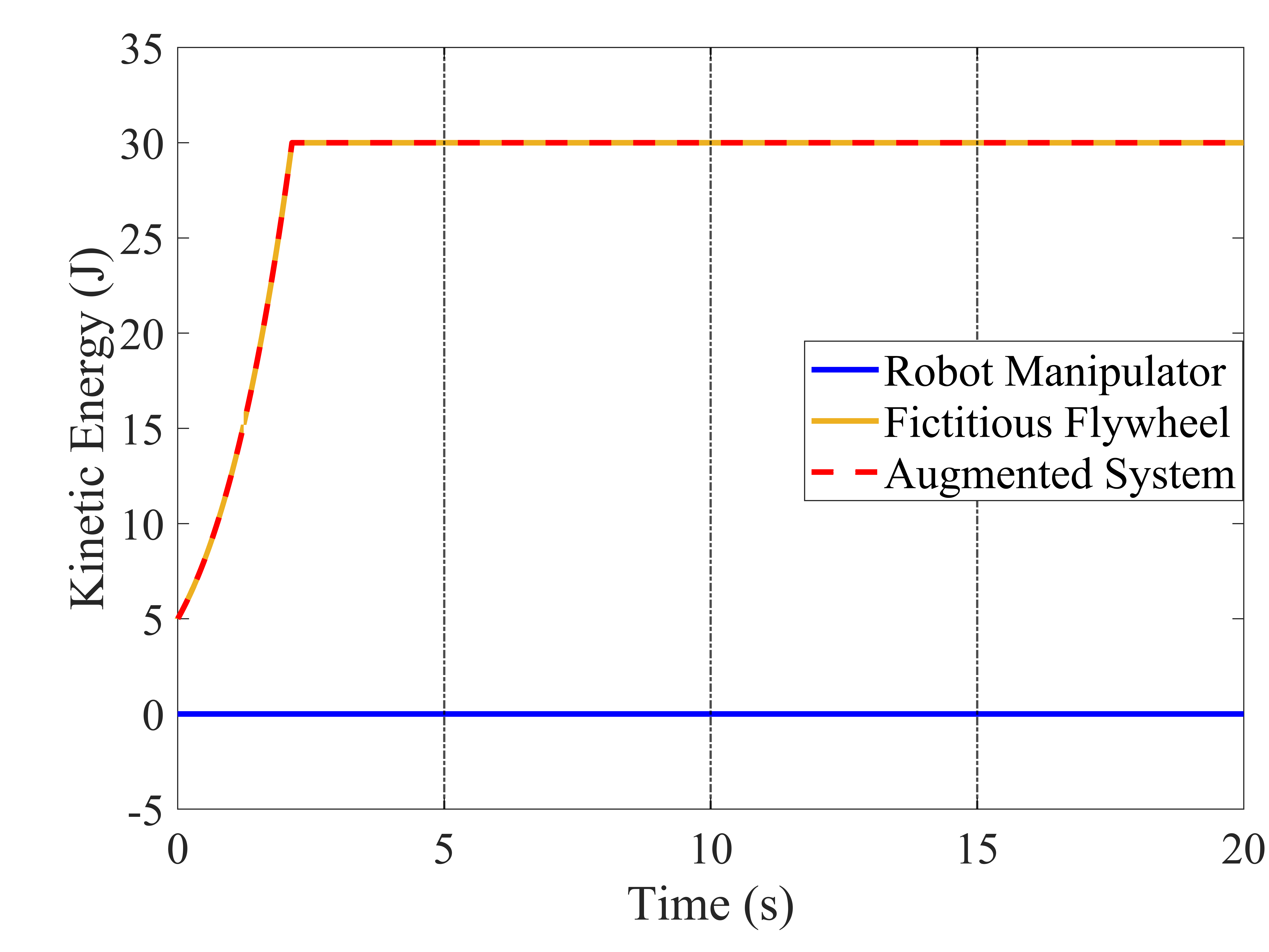
In Fig. 6, we focus on demonstrating the efficiency of the energy compensation mechanism within a finite time interval. Based on the computed settling time in (19), the control parameters are designed to guarantee the convergence of kinetic energy of the augmented system $\left({{k}^{a}}\left({{\mathbf{q}}^{a}},\,\,{{{\mathbf{\dot{q}}}}^{a}}\right)\right)$ to the desired level $\left(k_{d}^{a}=30\,\,\text{J}\right)$ within a specified timeframe. This feature presents a promising solution for time-critical applications, such as co-carrying fragile objects, in which precise control over the velocity of the robot partner and interaction force is imperative. According to (20) and (21), when the kinetic energy is insufficient, the robot partner’s movement rate is sluggish and cannot achieve the mutual tasks. On the contrary, safety violations may occur in co-carrying tasks when the robot partner moves too swiftly. In addition to maintaining the energy level, the relationship between the kinetic energy of the robot manipulator, fictitious flywheel, and augmented system is also described in Fig. 7.

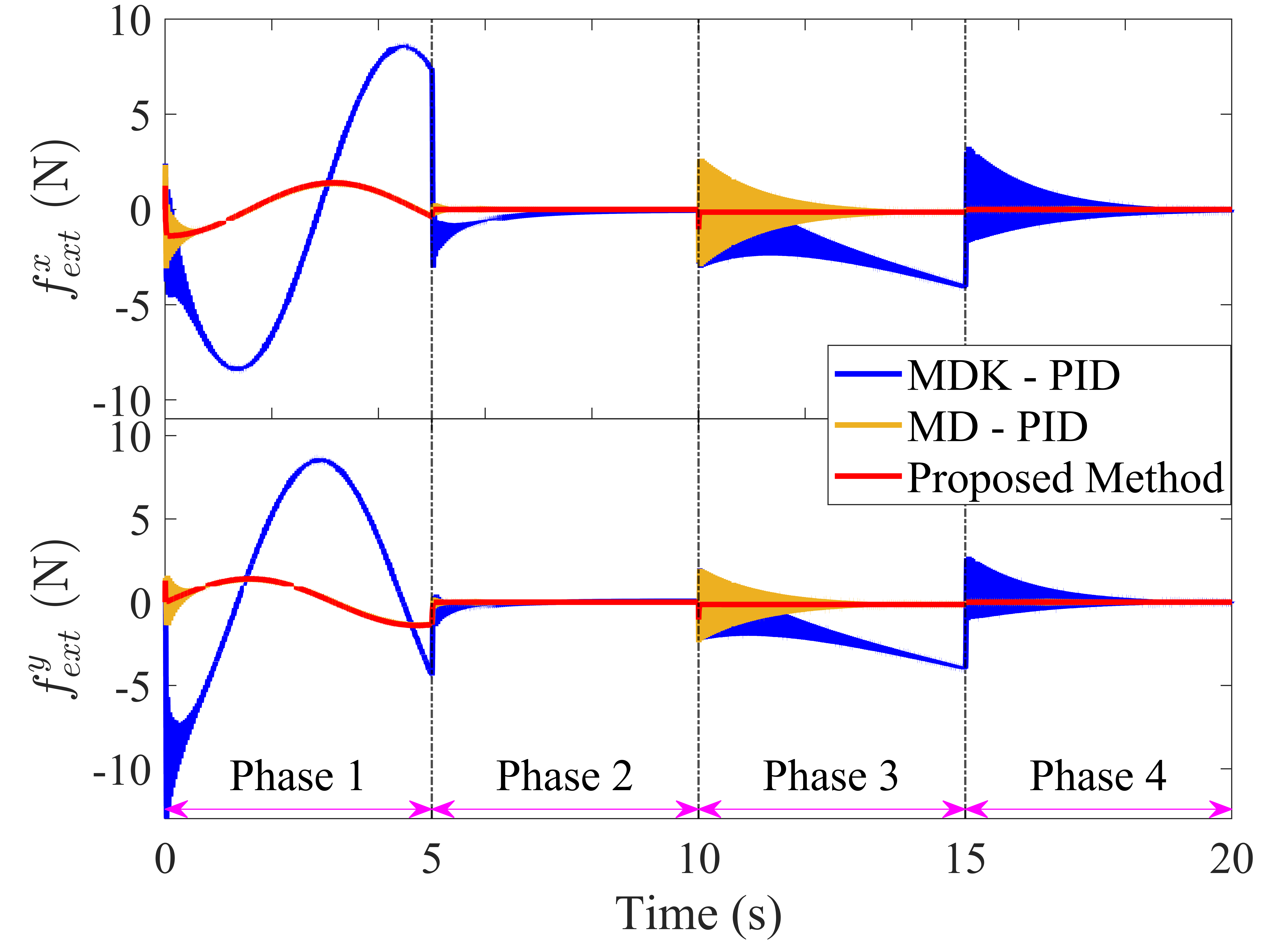
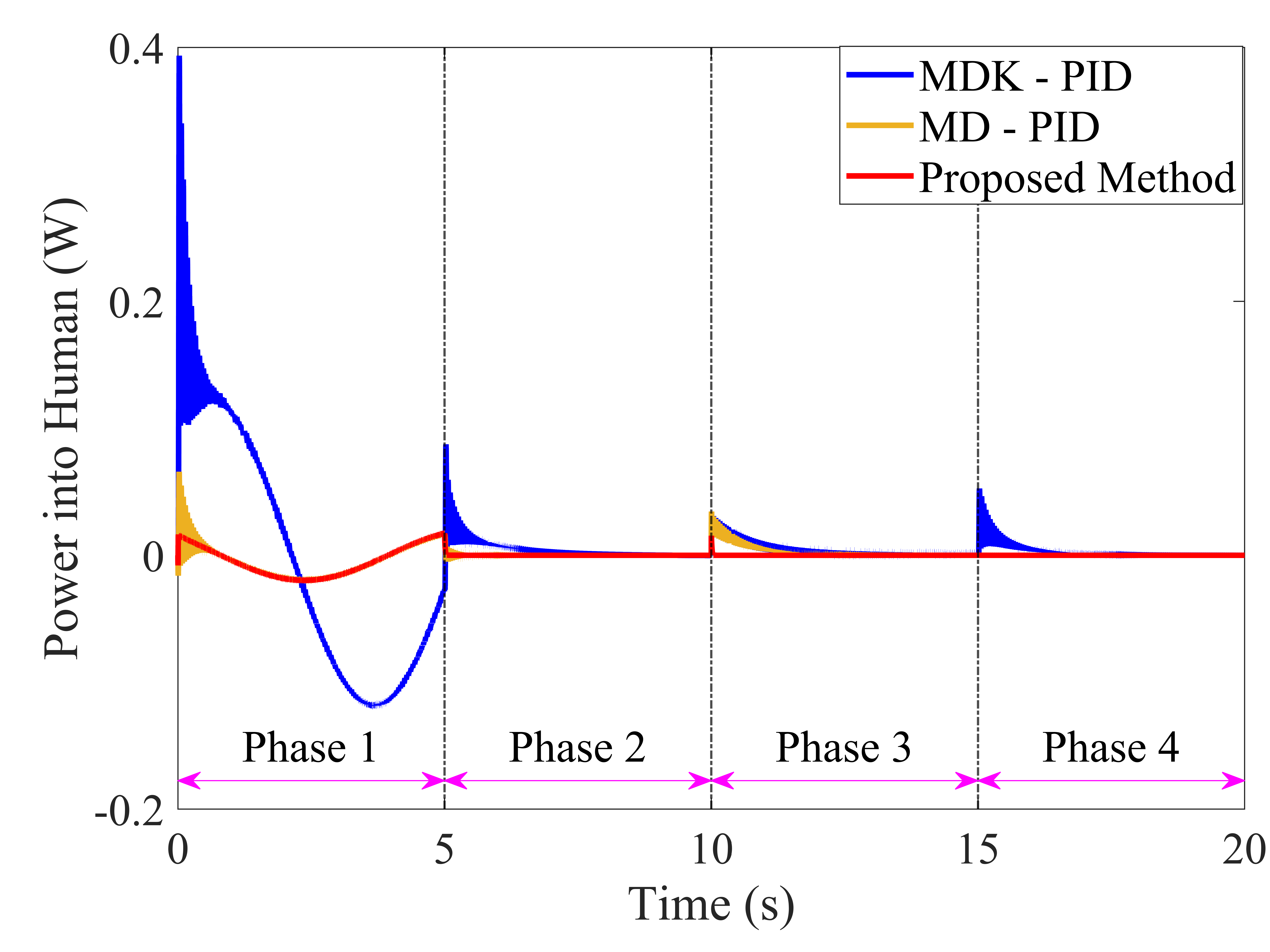
The human workload for the co-carrying task is exhibited by the human force in Fig. 8; meanwhile, the power flow into the human operator or co-transported object in (22) is also shown in Fig. 9. The chattering phenomenon of MDK-PID and MD-PID in Fig. 8 and Fig. 9 is caused by the responses of the position and velocity in (61) and (22). Furthermore, the volume of the human force and power of the Proposed Method is smaller than those in both the MDK-PID and MD-PID approaches in Phases 1 and 3. Meanwhile, during harmonious phases, the human force and power output of all three strategies approach zero, distinguishing them from the Admittance Model as,

{{\mathbf{M}}_{d}}{{{\mathbf{\ddot{x}}}}_{a}}+{{\mathbf{D}}_{d}}{{{\mathbf{\dot{x}}}}_{a}}={{\mathbf{f}}_{ext}}.

(66)

The Admittance Model in (66) utilizes ${{\mathbf{f}}_{ext}}$ as a trigger to generate movements, resulting in the presence of a certain level of human force and power even in harmonious phases. Consequently, the above Admittance Model in (66) presents challenges in manipulating fragile objects that necessitate a small external force $\left({{\mathbf{f}}_{ext}}\right)$ .

TABLE I: Average Data of Human Force and Power Flow into Human in Simulation Duration

Strategies	$f_{ext}^{x}\,\,\left(\text{N}\right)$	$f_{ext}^{y}\,\,\left(\text{N}\right)$	Power Flow $\left(\text{W}\right)$
MDK-PID	2.242	2.039	0.0250
MD-PID	0.467	0.453	0.0046
O-PVFC ${{\mathbf{K}}_{1}}=100{{\mathbf{I}}_{2\times 2}}$	_	_	_
O-PVFC ${{\mathbf{K}}_{1}}=10{{\mathbf{I}}_{2\times 2}}$	35.951	33.641	0.3721
Proposed Method	0.248	0.226	0.0028

Due to the significant magnitude of O-PVFC, the average data of four strategies is presented in Table I instead of being depicted in Figs. 3 - 9. To compare Human Force and Power Flow into Human, Table I is given by adopting the following formulation as

\text{Average=}\frac{1}{N}\sum\limits_{j=0}^{N=2000}{\left|\text{Dat}{{\text{a}}_{j}}\right|},

(67)

with $N$ is computed based on the simulation duration and time step of $20\,\text{s}$ and $0.01\,\text{s}$ , respectively. Based on the average data in Table I, it is quantitatively apparent that the values for the Proposed Method are approximately nine times smaller than those for the MDK-PID strategy and two times smaller than those for the MD-PID approach. For O-PVFC utilizing the same control parameters as those in the Proposed Method $\left({{\mathbf{K}}_{1}}=100{{\mathbf{I}}_{2\times 2}}\right)$ , the average data are not calculated because the simulation terminates abruptly at $1.52\,\text{s}$ . This implies that the time-varying Velocity Field of the robot manipulator increases continuously under the conflict in direction phase by the following expression,

\left\{\begin{aligned} &\mathbf{\dot{Q}}\left(t\right)={{\mathbf{J}}^{+}}\left(\mathbf{q}\right){{\mathbf{\dot{\hat{x}}}}_{h}}\left(t\right)\\ &\mathbf{V}\left(\mathbf{q},t\right)=\mathbf{\dot{Q}}\left(t\right)-{{\mathbf{K}}_{1}}\left(\mathbf{q}\left(t\right)-\mathbf{Q}\left(t\right)\right).\\ \end{aligned}\right.

(68)

As a result, the Velocity Field in (68) violates the existence condition of (9) due to $0.5{{\mathbf{V}}^{\top}}\left(\mathbf{q},t\right)\mathbf{M}\left(\mathbf{q}\right)\mathbf{V}\left(\mathbf{q},t\right)>{{E}^{a}}$ at $1.52\,\text{s}$ and the human–robot co-carrying task fails. By reducing the control parameter $\left({{\mathbf{K}}_{1}}=10{{\mathbf{I}}_{2\times 2}}\right)$ , O-PVFC resolved the simulation crashing problem in the case of ${{\mathbf{K}}_{1}}=100{{\mathbf{I}}_{2\times 2}}$ ; however, the substantial average magnitudes of Human Force and Power poses significant challenges for both co-carrying tasks and safe operations. Specifically, the Human Force and Power Flow into Human of the O-PVFC with ${{\mathbf{K}}_{1}}=10{{\mathbf{I}}_{2\times 2}}$ are roughly 147 and 115 times higher than those for the Proposed Method, respectively. In conclusion, the comparison results in Figs. 3 – 9 and average data in Table I not only demonstrated the superiority of the Proposed Method but also satisfied the requirements for human–robot co-carrying tasks including safe operation, varied human intentions, human–robot conflict, and human workload reduction.

V Discussion

This section answers the question ”Does the results of our cooperation control framework solve the problems discussed in Section II. A?” by comparing the proposed method with previous studies and analyzing its expandability to other human–robot collaboration scenarios. Finally, the limitations of the control framework are also discussed to clarify the application scope.

V-A Evaluation

On the one hand, utilizing the cooperation control framework in Section III. B with the results in III. C resolved three problems (P1)–(P3) listed in Section II. A. For the first problem in (P1), leveraging the admittance property, the robot partner proactively follows the human intention in harmonious movement scenarios, resulting in human workload reduction. Meanwhile, in noteworthy situations such as the conflict in direction and parking location, the co-carrying path is re-planned for the robot according to human–robot interaction forces. For safe operation, the results in Theorem 1 and Lemma 3 are presented to guarantee the passivity of the closed-loop system under ${{k}^{a}}\left({{\mathbf{q}}^{a}},{{{\mathbf{\dot{q}}}}^{a}}\right)\geq k_{d}^{a}$ . Moreover, the power flow into the human operator, robot partner, and co-transported object can be reduced. Furthermore, energy compensation capacity within a finite time interval in Theorem 2 is necessary for time-critical applications. Based on (20) and (21), if the amount of the kinetic energy is significantly small, the moving rate of the robot partner is slow and hence, the robot cannot achieve the mutual tasks. By contrast, safety in co-carrying tasks can be violated when the robot partner moves at a fast rate. Thus, the second problem (P2) was addressed by using the analysis in Theorems 1, 2, and Lemma 3. Last but not least, the tracking problem of the time-varying co-carrying task in (P3) was resolved by our cooperation control framework with the result in Theorem 3; therefore, the human–robot co-carrying tasks were completed.

On the other hand, the numerical simulation results in Section IV. B demonstrated the effectiveness of the proposed cooperation control framework in Sections III. B, C. In Figs. 4 and 5, by re-planning the co-carrying trajectory based on conflict information, the robot partner can follow human motion intentions in conflict phases. Meanwhile, in two harmonious movement phases, the robot partner proactively and accurately tracks the estimated human intentions. The control and compensation for the energy of the closed-loop system within a finite time interval are depicted in Fig. 6 and Fig. 7. Through the amount of the interaction forces and power flow shown in Figs. 8, 9, and Table I, the proposed method underscores the capacity of human workload reduction and human–robot power flow management, especially in human–robot conflicts phases. Thus, the above simulation results and analysis further reinforced the significance of integrating admittance control and time-varying PVFC with a fractional exponent energy compensation control term in addressing the problems in Section II. A.

V-B Comparison

Comparing our proposed framework with the cooperation control method in [9], we see that our framework ensures continuous transfer between interaction states by utilizing human–robot interaction forces, which is formulated in (7). Meanwhile, the approach in [9] switches between interaction states based on their exact characteristics, resulting in unstable behavior at switching points and posing challenges for practical applications due to the complexity of distinguishing between states. In [22], admittance control was adopted as defined (66), which consistently necessitates human forces for co-carrying movement. In contrast to this study, equation (7) and Fig. 8 demonstrated that the human forces in our method are zero in the harmonious movement phases, thereby reducing human workload. Moreover, the time-varying PVFC in (12) is supplemented by the fractional exponent energy compensation control term, which is not considered in [30, 32, 33]. Our approach comprehensively investigates the variable kinetic energy instead of only focusing on ${{k}^{a}}\left({{\mathbf{q}}^{a}},{{{\mathbf{\dot{q}}}}^{a}}\right)\leq k_{d}^{a}$ in [32]. In comparison with the study with a special case $\left(\frac{{{r}_{1}}}{{{r}_{2}}}=1\right)$ in [33], we investigate the fractional-order algorithm in our proposed framework to determine the convergence time of the kinetic energy. Furthermore, the difference between the proposed strategy and those in [30, 32, 33] is the consideration of the position error and time-varying Velocity Field, which qualifies for human–robot co-carrying tasks.

V-C Scalability

The human–robot co-carrying tasks is a specific application of our cooperation control framework. It is expected to be scalable for other human–robot cooperation tasks such as handover, assembly, teleoperation, sawing, and so on. To come up with the statement, similar design characteristics and technique requirements are detected for the human–robot cooperation scheme.

•

First, human–robot cooperation control strategies are developed for robot manipulators to assist the human operator in common tasks. Therefore, determining accordant movement for the robot partner in the interaction phase is a critical function in synchronizing human–robot movements of the aforementioned scenarios. Furthermore, the energy and power in human–robot systems have to be considered to minimize the potential risk of harm to the human operator and robot. Regarding the human–robot collaboration handover, assembly, and teleoperation applications, the independent working phase without human–robot interaction would also have to be included. It is necessary to supplement an autonomous mode, which will be processed by our new PVFC.
•

Second, human workload reduction, human–robot conflict resolution, and safety interaction are considered common technical requirements for human–robot collaboration systems. According to the results in Section III. C and analyses in Section III. E, the technical requirements are guaranteed by the proposed method. Thus, the advantages of our cooperation control framework can be extended to other human–robot collaboration applications in a straightforward manner.

V-D Limitation

The present study focused on the human–robot co-carrying task for a small transported object on a horizontal surface. Therefore, the effects of gravity were ignored and it was assumed that the position of the human hand was similar to the end-effector position of the robot arm. Although our cooperation control framework was developed by utilizing the aforementioned assumptions, this will only impact the results in the case of co-carrying large or heavy objects. Directly applying our proposed framework to large or heavy objects may not yield the efficiencies and performances observed in our co-carrying scenarios. We thus plan to investigate a human–robot collaboration approach for large or heavy objects in future works, discarding the above assumptions.

VI CONCLUSION AND FUTURE WORK

In this paper, a cooperation control framework using admittance control and new time-varying PVFC was proposed and applied for human–robot co-carrying tasks. Admittance control was employed to re-plan the co-carrying trajectory for the robot manipulator when conflicts in movements between a human and a robot were detected by the interaction force. A new PVFC with a fractional exponent control term was developed to guarantee the passivity of the closed-loop system, compensate for the kinetic energy within a finite time interval, reduce power flow from the robot to the human, and track the co-carrying path. The proposed method was validated by comparative simulation under four collaboration conditions, including conflict in direction and parking location, and two harmonious movement phases.

To enhance the flexibility of the cooperation control framework, a prediction method will be considered and developed for calculating future human motion intentions. Furthermore, the proposed cooperation control method needs to be extended to be applicable to other human-robot cooperation systems such as handover, assembly, teleoperation, sawing, and so on in upcoming work. In this study, experimental evaluations in a real robotic system have not been presented and investigated. Therefore, it will be necessary to validate the efficiency of the proposed approach for human-robot collaboration systems through experimental viewpoints in future work.

References

[1] M. A. B. Mohammed Zaffir and T. Wada, “Presentation of robot-intended handover position using vibrotactile interface during robot-to-human handover task,” in Proceedings of the 2024 ACM/IEEE International Conference on Human-Robot Interaction, 2024, pp. 492–500.
[2] X. Yu, B. Li, W. He, Y. Feng, L. Cheng, and C. Silvestre, “Adaptive-constrained impedance control for human–robot co-transportation,” IEEE transactions on cybernetics, vol. 52, no. 12, pp. 13 237–13 249, 2021.
[3] E. Ng, Z. Liu, and M. Kennedy, “It takes two: Learning to plan for human-robot cooperative carrying,” in 2023 IEEE International Conference on Robotics and Automation (ICRA). IEEE, 2023, pp. 7526–7532.
[4] M. Ma and L. Cheng, “A human–robot collaboration controller utilizing confidence for disagreement adjustment,” IEEE Transactions on Robotics, vol. 40, pp. 2081–2097, 2024.
[5] Z. Al-Saadi, D. Sirintuna, A. Kucukyilmaz, and C. Basdogan, “A novel haptic feature set for the classification of interactive motor behaviors in collaborative object transfer,” IEEE Transactions on Haptics, vol. 14, no. 2, pp. 384–395, 2020.
[6] H. L. Thi, V. T. Dang, N. T. Nguyen, D. T. Le, and T. L. Nguyen, “A neural network-based fast terminal sliding mode controller for dual-arm robots,” in International Conference on Engineering Research and Applications. Springer, 2022, pp. 42–52.
[7] X. Zhao, Y. Zhang, W. Ding, B. Tao, and H. Ding, “A dual-arm robot cooperation framework based on a nonlinear model predictive cooperative control,” IEEE/ASME Transactions on Mechatronics, 2023.
[8] A. Pervez and J. Ryu, “Safe physical human robot interaction-past, present and future,” Journal of Mechanical Science and Technology, vol. 22, pp. 469–483, 2008.
[9] Z. Al-Saadi, Y. M. Hamad, Y. Aydin, A. Kucukyilmaz, and C. Basdogan, “Resolving conflicts during human-robot co-manipulation,” in Proceedings of the 2023 ACM/IEEE International Conference on Human-Robot Interaction, 2023, pp. 243–251.
[10] X. Yu, W. He, Y. Li, C. Xue, J. Li, J. Zou, and C. Yang, “Bayesian estimation of human impedance and motion intention for human–robot collaboration,” IEEE transactions on cybernetics, vol. 51, no. 4, pp. 1822–1834, 2019.
[11] D. J. Agravante, A. Cherubini, A. Bussy, P. Gergondet, and A. Kheddar, “Collaborative human-humanoid carrying using vision and haptic sensing,” in 2014 IEEE international conference on robotics and automation (ICRA). IEEE, 2014, pp. 607–612.
[12] X. Yu, W. He, Q. Li, Y. Li, and B. Li, “Human-robot co-carrying using visual and force sensing,” IEEE Transactions on Industrial Electronics, vol. 68, no. 9, pp. 8657–8666, 2020.
[13] C. Ott, R. Mukherjee, and Y. Nakamura, “Unified impedance and admittance control,” in 2010 IEEE international conference on robotics and automation. IEEE, 2010, pp. 554–561.
[14] N. Hogan, “Impedance control: An approach to manipulation: Part i—theory,” Journal of Dynamic Systems Measurement and Control-transactions of The Asme, vol. 107, pp. 1–7, 1985.
[15] C. Ott, R. Mukherjee, and Y. Nakamura, “A hybrid system framework for unified impedance and admittance control,” Journal of Intelligent & Robotic Systems, vol. 78, pp. 359–375, 2015.
[16] T. Fujiki and K. Tahara, “Series admittance–impedance controller for more robust and stable extension of force control,” ROBOMECH Journal, vol. 9, no. 1, p. 23, 2022.
[17] J. Luo, C. Zhang, W. Si, Y. Jiang, C. Yang, and C. Zeng, “A physical human–robot interaction framework for trajectory adaptation based on human motion prediction and adaptive impedance control,” IEEE Transactions on Automation Science and Engineering, pp. 1–12, 2024.
[18] Y. Dong, W. He, L. Kong, and X. Hua, “Impedance control for coordinated robots by state and output feedback,” IEEE Transactions on Systems, Man, and Cybernetics: Systems, vol. 51, no. 8, pp. 5056–5066, 2021.
[19] Z. Li, X. Li, Q. Li, H. Su, Z. Kan, and W. He, “Human-in-the-loop control of soft exosuits using impedance learning on different terrains,” IEEE Transactions on Robotics, vol. 38, no. 5, pp. 2979–2993, 2022.
[20] X. Xing, E. Burdet, W. Si, C. Yang, and Y. Li, “Impedance learning for human-guided robots in contact with unknown environments,” IEEE Transactions on Robotics, 2023.
[21] M. Sharifi, A. Zakerimanesh, J. K. Mehr, A. Torabi, V. K. Mushahwar, and M. Tavakoli, “Impedance variation and learning strategies in human–robot interaction,” IEEE Transactions on Cybernetics, vol. 52, no. 7, pp. 6462–6475, 2022.
[22] C. T. Landi, F. Ferraguti, L. Sabattini, C. Secchi, and C. Fantuzzi, “Admittance control parameter adaptation for physical human-robot interaction,” in 2017 IEEE international conference on robotics and automation (ICRA). IEEE, 2017, pp. 2911–2916.
[23] M. Khoramshahi and A. Billard, “A dynamical system approach for detection and reaction to human guidance in physical human–robot interaction,” Autonomous Robots, vol. 44, no. 8, pp. 1411–1429, 2020.
[24] D. Sirintuna, A. Giammarino, and A. Ajoudani, “Human-robot collaborative carrying of objects with unknown deformation characteristics,” in 2022 IEEE/RSJ International Conference on Intelligent Robots and Systems (IROS). IEEE, 2022, pp. 10 681–10 687.
[25] D. Sirintuna, I. Ozdamar, and A. Ajoudani, “Carrying the uncarriable: a deformation-agnostic and human-cooperative framework for unwieldy objects using multiple robots,” in 2023 IEEE International Conference on Robotics and Automation (ICRA). IEEE, 2023, pp. 7497–7503.
[26] D. Lee and P. Y. Li, “Passive bilateral feedforward control of linear dynamically similar teleoperated manipulators,” IEEE Transactions on Robotics and Automation, vol. 19, no. 3, pp. 443–456, 2003.
[27] F. Benzi, F. Ferraguti, G. Riggio, and C. Secchi, “An energy-based control architecture for shared autonomy,” IEEE Transactions on Robotics, vol. 38, no. 6, pp. 3917–3935, 2022.
[28] Y. Michel, C. Ott, and D. Lee, “Safety-aware hierarchical passivity-based variable compliance control for redundant manipulators,” IEEE Transactions on Robotics, vol. 38, no. 6, pp. 3899–3916, 2022.
[29] F. Ferraguti, N. Preda, A. Manurung, M. Bonfè, O. Lambercy, R. Gassert, R. Muradore, P. Fiorini, and C. Secchi, “An energy tank-based interactive control architecture for autonomous and teleoperated robotic surgery,” IEEE Transactions on Robotics, vol. 31, no. 5, pp. 1073–1088, 2015.
[30] P. Y. Li and R. Horowitz, “Passive velocity field control of mechanical manipulators,” IEEE Transactions on robotics and automation, vol. 15, no. 4, pp. 751–763, 1999.
[31] P. Li and R. Horowitz, “Passive velocity field control (pvfc). part i. geometry and robustness,” IEEE Transactions on Automatic Control, vol. 46, no. 9, pp. 1346–1359, 2001.
[32] T. Shogaki, T. Wada, and Y. Fukui, “Velocity field control with energy compensation toward therapeutic exercise,” in 2014 IEEE International Conference on Robotics and Biomimetics (ROBIO 2014). IEEE, 2014, pp. 1572–1577.
[33] Y. Fukui and T. Wada, “Velocity field control with energy compensation toward therapeutic exercise,” in 2016 IEEE 55th Conference on Decision and Control (CDC). IEEE, 2016, pp. 835–842.
[34] C. Secchi, S. Stramigioli, and C. Fantuzzi, Control of interactive robotic interfaces: A port-Hamiltonian approach. Springer Science & Business Media, 2007, vol. 29.
[35] X. Huang, W. Lin, and B. Yang, “Global finite-time stabilization of a class of uncertain nonlinear systems,” Automatica, vol. 41, no. 5, pp. 881–888, 2005.
[36] W. M. Haddad and V. Chellaboina, Nonlinear Dynamical Systems and Control: A Lyapunov-Based Approach. Princeton University Press, 2008.
[37] H. Khalil, Nonlinear Systems, ser. Pearson Education. Prentice Hall, 2002.
[38] J.-J. E. Slotine, W. Li et al., Applied nonlinear control. Prentice hall Englewood Cliffs, NJ, 1991, vol. 199, no. 1.