A Convex Parameterization of Robust Recurrent Neural Networks

Max Revay, Ruigang Wang, Ian R. Manchester This work was supported by the Australian Research Council.The authors are with the Australian Centre for Field Robotics, The University of Sydney, Sydney, NSW 2006, Australia (e-mail: [email protected]).

Abstract

Recurrent neural networks (RNNs) are a class of nonlinear dynamical systems often used to model sequence-to-sequence maps. RNNs have excellent expressive power but lack the stability or robustness guarantees that are necessary for many applications. In this paper, we formulate convex sets of RNNs with stability and robustness guarantees. The guarantees are derived using incremental quadratic constraints and can ensure global exponential stability of all solutions, and bounds on incremental $\ell_{2}$ gain (the Lipschitz constant of the learned sequence-to-sequence mapping). Using an implicit model structure, we construct a parametrization of RNNs that is jointly convex in the model parameters and stability certificate. We prove that this model structure includes all previously-proposed convex sets of stable RNNs as special cases, and also includes all stable linear dynamical systems. We illustrate the utility of the proposed model class in the context of non-linear system identification.

I INTRODUCTION

RNNs are state-space models incorporating neural networks that are frequently used in system identification and machine learning to model dynamical systems and other sequences-to-sequence mappings. It has long been observed that RNNs can be difficult to train in part due to model instability, referred to as the exploding gradients problem [1], and recent work shows that these models are often not robust to input perturbations [2]. These issues are related to long-standing concerns in control theory, i.e. stability and Lipschitz continuity solutions of dynamical systems [3].

There are many types of stability for nonlinear systems (e.g., RNNs). When learning dynamical systems with inputs, Lyapunov approaches are inappropriate as they require the construction of a Lyapunov function about a known stable solution. In machine learning and system identification, however, the goal is to simulate the learned model with new inputs, generating new solutions. Incremental stability [4] and contraction analysis [5] avoid this issue by showing stability for all inputs and trajectories.

Even if a model is stable, it is usually problematic if its output is very sensitive to small changes in the input. This sensitivity can be quantified by the model’s incremental $\ell_{2}$ gain. Finite incremental $\ell_{2}$ gain implies both boundedness and continuity of the input-output map [4]. Furthermore, the incremental $\ell_{2}$ gain bound is also a bound on the Lipschitz constant of the sequence-to-sequence mapping. In machine learning, the Lipschitz constant is used in proofs of generalization bounds [6], analysis of expressiveness [7] and guarantees of robustness to adversarial attacks [8, 9].

The problem of training models with stability or robustness guaranteed a-priori has seen significant attention for both linear [10, 11] and nonlinear [12, 13, 14] models. The main difficult comes from the non-convexity of most model structures and their stability certificates. Some methods deal with this difficulty by simply fixing the stability certificate and optimizing over the model parameters at significant cost to model expressibility [15]. It has recently been shown that implicit parametrizations allow joint convexity of the model and a stability certificate for linear [16], polynomial [12] and RNN [17] models. It has been observed that stability constraints serve as an effective regulariser and can improve generalisation performance [18, 17].

When a system is expressed in terms of a neural network, even the problem of analyzing the stability of known dynamics is difficult. A number of approaches have formulated LMI conditions [19, 20, 21] guaranteeing Lyapunov stability of a particular equilibrium. Recently, incremental quadratic constraints [3] have been recently applied to (non-recurrent) neural networks to develop the tightest bounds on the Lipschitz constant known to date [22].

Contributions: In this letter we propose a new convex parameterization of RNNs satisfying stability and robustness conditions. By treating RNNs as linear systems in feedback with a slope-restricted, element-wise nonlinearity, we can apply methods from robust control to develop stability conditions that are less conservative than prior methods. The proposed model set contains all previously published sets of stable RNNs, and all stable linear time-invariant (LTI) systems. Using implicit parameterizations with incremental quadratic constraints, we construct a set of models that is jointly convex in the model parameters, stability certificate and the multipliers required by the incremental quadratic constraint approach. Joint convexity in all parameters simplifies the training of stable models as constraints can be easily dealt with using penalty, barrier or projected gradient methods.

Notation. We use $\mathbb{N},\mathbb{R}$ to denote the set of natural and real numbers, respectively. The set of all one-side sequences $x:\mathbb{N}\rightarrow\mathbb{R}^{n}$ is denoted by $\ell_{2e}^{n}$ . Superscript $n$ is omitted when it is clear from the context. For $x\in\ell_{2e}^{n}$ , $x_{t}\in\mathbb{R}^{n}$ is the value of the sequence $x$ at time $t\in\mathbb{N}$ . The notation $|\cdot|:\mathbb{R}^{n}\rightarrow\mathbb{R}$ denotes the standard 2-norm. The subset $\ell_{2}\subset\ell_{2e}$ consists of all square-summable sequences, i.e., $x\in\ell_{2}$ if and only if the $\ell_{2}$ norm $\|x\|:=\sqrt{\sum_{t=0}^{\infty}|x_{t}|^{2}}$ is finite. Given a sequence $x\in\ell_{2e}$ , the $\ell_{2}$ norm of its truncation over $[0,T]$ with $T\in\mathbb{N}$ is written as $\|x\|_{T}:=\sqrt{\sum_{t=0}^{T}|x_{t}|^{2}}$ . For matrices $A$ , we use $A\succ 0$ and $A\succeq 0$ to mean $A$ is positive definite or positive semi-definite respectively and $A\succ B$ and $A\succeq 0$ to mean $A-B\succ 0$ and $A-B\succeq 0$ respectively. The set of diagonal, positive definite matrices is denoted $\mathbb{D}_{+}$ .

II Problem Formulation

We are interested in learning nonlinear state space models:

	$\displaystyle x_{t+1}=f_{\theta}(x_{t},u_{t}),$		(1)
	$\displaystyle y_{t}=g_{\theta}(x_{t},u_{t}),$		(2)

where $x_{t}\in\mathbb{R}^{n}$ is the state, $u_{t}\in\mathbb{R}^{m}$ is a known input and $y_{t}\in\mathbb{R}^{p}$ is the output. The functions $f_{\theta},g_{\theta}$ are parametrized by $\theta\in\Theta\subseteq\mathbb{R}^{N}$ and will be defined later. Given initial condition $x_{0}=a$ , the dynamical system (1), (2) can be provides a sequence-to-sequence mapping $S_{a}:\ell_{2e}^{m}\mapsto\ell_{2e}^{p}$ .

Definition 1.

The system (1), (2) is termed incrementally $\ell_{2}$ stable if for any two initial conditions $a$ and $b$ , given the same input sequence $u$ , the corresponding output trajectories $y^{a}$ and $y^{b}$ satisfy $y^{a}-y^{b}\in\ell_{2}^{p}$ .

This definition implies that initial conditions are forgotten, however, the outputs can still be sensitive to small perturbations in the input. In such cases, it is natural to measure system robustness in terms of the incremental $\ell_{2}$ -gain.

Definition 2.

The system (1), (2) is said to have an incremental $\ell_{2}$ -gain bound of $\gamma$ if for all pairs of solutions with initial conditions $a,b\in\mathbb{R}^{n}$ and input sequences $u^{a},u^{b}\in\ell_{2e}^{m}$ , the output sequences $y^{a},y^{b}\in\ell_{2e}^{p}$ satisfy

\left\|y^{a}-y^{b}\right\|_{T}^{2}\leq\gamma^{2}\left\|u^{a}-u^{b}\right\|_{T}^{2}+d(a,b),\quad\forall T\in\mathbb{N},

(3)

for some $d(a,b)\geq 0$ with $d(a,a)=0$ .

Note that the above definition implies incremental $\ell_{2}$ stability since $\|y^{a}-y^{b}\|_{T}^{2}\leq d(a,b)$ for all $T\in\mathbb{N}$ when $u^{a}=u^{b}$ . It also shows that all operators defined by (1) and (2) are Lipschitz continuous with Lipschitz constant $\gamma$ , i.e. for any $a\in\mathbb{R}^{n}$ and all $T\in\mathbb{N}$

\|S_{a}(u)-S_{a}(v)\|_{T}\leq\gamma\|u-v\|_{T},\quad\forall u,v\in\ell_{2e}^{m}.

(4)

The goal of this work is to construct a rich parametrization of the functions $f_{\theta}$ and $g_{\theta}$ in (1), (2), with robustness guarantees. We focus on two robustness guarantees in this work:

1.

A model set parametrized by $\Theta_{*}\subset R^{N}$ is robust if for all $\theta\in\Theta_{*}$ the system has finite incremental $\ell_{2}$ -gain.
2.

A model set parameterized by $\Theta_{\gamma}\subset R^{N}$ is $\gamma$ -robust if for all $\theta\in\Theta_{\gamma}$ the system has an incremental $\ell_{2}$ -gain bound of $\gamma$ .

III Robust RNNs

III-A Model Structure

Refer to caption — Figure 1: Feedback interconnection for RNNs.

We parameterize the functions (1), (2) as a feedback interconnection between a linear system $G$ and a static, memoryless nonlinear operator $\Phi$ :

	$\displaystyle G\;\begin{cases}x_{t+1}=\bar{F}x_{t}+\bar{B}_{1}w_{t}+\bar{B}_{2}u_{t}\\ y_{t}=C_{1}x_{t}+D_{11}w_{t}+D_{12}u_{t}\\ v_{t}=\bar{C}_{2}x_{t}+\bar{b}+\bar{D}_{22}u_{t}\end{cases},$		(5)
	$\displaystyle w=\Phi(v),$		(6)

where $\Phi(v)=[\phi(v_{1})\ \cdots\ \phi(v_{q})]^{\top}$ with $v_{i}$ as the $i$ th component of the $v\in\ell_{2e}^{q}$ . This feedback interconnection is shown in Fig. 1. We assume that the slope of $\phi$ is restricted to the interval $[0,\beta]$ :

0\leq\frac{\phi(y)-\phi(x)}{y-x}\leq\beta,\quad\forall x,y\in\mathbb{R},~{}x\neq y.

(7)

In the neural network literature, such functions are referred to as “activation functions”, and common choices (e.g. tanh, ReLU, sigmoid) are slope restricted [23].

The proposed model structure is highly expressive and contains many commonly used model structures. For instance, LTI systems are obtained when $\bar{B}_{1}=0$ and $D_{11}=0$ . RNNs of the form [24]:

	$\displaystyle x_{t+1}=\mathcal{B}_{1}\Phi(\mathcal{A}x_{t}+\mathcal{B}u_{t}+b),$		(8)
	$\displaystyle y_{t}=\mathcal{C}x_{t}+\mathcal{D}u_{t},$		(9)

are obtained with the choice $\bar{F}=0$ , $\bar{B}_{1}=\mathcal{B}_{1}$ , $\bar{B}_{2}=0$ , $C_{1}=\mathcal{C}$ , $D_{11}=0$ , $D_{12}=\mathcal{D}$ , $\bar{C}_{2}=\mathcal{A}$ , $\bar{D}_{22}=\mathcal{B}$ and $\bar{b}=b$ . This implies (5), (6) is a universal approximator for dynamical systems over bounded domains as $q\rightarrow\infty$ [25].

Even for linear systems, the set of robust or $\gamma$ -robust models is non-convex. Constructing a set of parameters for which (5), (6) is robust or $\gamma$ -robust is further complicated by presence of the nonlinear activation function in $\Phi$ . We will simplify the analysis by replacing $\Phi$ with incremental quadratic constraints.

III-B Description of $\Phi$ by Incremental Quadratic Constraints

Multiplying (7) through by $(y-x)^{2}$ , and combining the two inequalities, we get:

\left[\begin{matrix}y-x\\ \phi(y)-\phi(x)\end{matrix}\right]^{\top}\left[\begin{matrix}0&\beta\\ \beta&-2\end{matrix}\right]\left[\begin{matrix}y-x\\ \phi(y)-\phi(x)\end{matrix}\right]\geq 0.

(10)

For $v^{a},v^{b}\in\mathbb{R}^{q}$ and $w^{a}=\Phi(v^{a})$ , $w^{b}=\Phi(v^{b})$ , (10) holds for each element with $y=v^{a}_{i}$ and $x=v^{b}_{i}$ . Taking a conic combination of these constraints with multipliers $\lambda_{i}>0$ , we get:

\displaystyle\begin{bmatrix}v^{a}_{t}-v^{b}_{t}\\ w^{a}_{t}-w^{b}_{t}\end{bmatrix}^{\top}\underset{M(\Lambda)}{\underbrace{\begin{bmatrix}0&\beta\Lambda\\ \beta\Lambda&-2\Lambda\end{bmatrix}}}\begin{bmatrix}v^{a}_{t}-v^{b}_{t}\\ w^{a}_{t}-w^{b}_{t}\end{bmatrix}\geq 0,

(11)

where $\Lambda=\mathrm{diag}(\lambda_{1},...,\lambda_{q})$ .

III-C Convex Parametrization of Robust RNNs

Corresponding to the linear system (5), we introduce the following implicit, redundant parametrization:

G\;\begin{cases}Ex_{t+1}=Fx_{t}+B_{1}w_{t}+B_{2}u_{t}\\ y_{t}=C_{1}x_{t}+D_{11}w_{t}+D_{12}u_{t}\\ \Lambda v_{t}=C_{2}x_{t}+b+D_{22}u_{t}\end{cases}

(12)

where $\theta=(E,F,B_{1},B_{2},C_{1},D_{11},D_{12},\Lambda,C_{2},b,D_{22})$ are the model parameters with $E$ invertible and $\Lambda\in\mathbb{D}_{+}$ is the incremental quadratic constraint multiplier from (11). The explicit system (5) can be easily constructed from (12) by inverting $E$ and $\Lambda$ . While the parameters $E$ and $\Lambda$ do not improve model expressiveness, the extra degrees of freedom will allow us to formulate sets of robust models that are jointly convex in the model parameters, stability certificate and multipliers.

To construct the set of stable robust models, we introduce the following convex constraint:

\begin{bmatrix}E+E^{\top}-P&-\beta{C}^{\top}_{2}\\ -\beta{C}_{2}&2\Lambda\end{bmatrix}-\begin{bmatrix}{F}^{\top}\\ {B}_{1}^{\top}\end{bmatrix}P^{-1}\begin{bmatrix}{F}^{\top}\\ {B}_{1}^{\top}\end{bmatrix}^{\top}\succ 0,

(13)

The set of Robust RNNs is then given by:

\Theta_{*}:=\{\theta:\exists P\succ 0,\,\Lambda\in\mathbb{D}_{+}\;\mathrm{s.t.}\;\eqref{eq:bound_l2_gain_lmi}\}.

Since $P\succ 0$ , (13) and (14) imply that $E+E^{\top}\succ 0$ which means that $E$ is invertible.

To construct a set of $\gamma$ -robust models, we propose the following convex constraint:

\begin{bmatrix}E+E^{\top}-P&-\beta{C}_{2}^{\top}&0\\ -\beta{C}_{2}&2\Lambda&-\beta{D}_{22}^{\top}\\ 0&-\beta{D}_{22}&\gamma I\end{bmatrix}\\ -\begin{bmatrix}F^{\top}\\ B_{1}^{\top}\\ B_{2}^{\top}\end{bmatrix}P^{-1}\begin{bmatrix}F^{\top}\\ B_{1}^{\top}\\ B_{2}^{\top}\end{bmatrix}^{\top}-\frac{1}{\gamma}\begin{bmatrix}C_{1}^{\top}\\ D_{11}^{\top}\\ D_{12}^{\top}\end{bmatrix}\begin{bmatrix}C_{1}^{\top}\\ D_{11}^{\top}\\ D_{12}^{\top}\end{bmatrix}^{\top}\succ 0,

(14)

The set of $\gamma$ -robust RNNs is then given by:

\Theta_{\gamma}:=\{\theta:\exists P\succ 0,\,\Lambda\in\mathbb{D}_{+}\;\mathrm{s.t.}\;\eqref{eq:dl2_gain_bound_lmi}\}.

Note that (13) and (14) are jointly convex in the model parameters, stability certificate, multipliers $\Lambda$ and the incremental $\ell_{2}$ gain bound $\gamma$ .

Theorem 1.

Suppose that $\theta\in\Theta_{\gamma}$ , then the Robust RNN (5), (6) has a incremental $\ell_{2}$ -gain bound of $\gamma$ .

Proof.

Consider two solutions $x^{a},x^{b}\in\ell_{2e}^{n}$ and outputs $y^{a},y^{b}\in\ell_{2e}^{p}$ to the system (1), (2) with initial conditions $a,b\in\mathbb{R}^{n}$ and inputs $u^{a},u^{b}\in\ell_{2e}^{m}$ . Let $\Delta u=u^{a}-u^{b}$ , $\Delta x=x^{a}-x^{b}$ , $\Delta v=v^{a}-v^{b}$ , $\Delta w=w^{a}-w^{b}$ and $\Delta y=y^{a}-y^{b}$ .

To establish the incremental $\ell_{2}$ -gain bound, we first left and right multiply (14) by the vectors $\left[\begin{matrix}\Delta x_{t}^{\top},\Delta w_{t}^{\top},\Delta u_{t}^{\top}\end{matrix}\right]$ and $\left[\begin{matrix}\Delta{x_{t}}^{\top},\Delta{w_{t}}^{\top},\Delta{u_{t}}^{\top}\end{matrix}\right]^{\top}$ . Applying the bound $-E^{\top}P^{-1}E\preceq P-E-E^{\top}$ [12] and introducing the storage function $V_{t}=\Delta x_{t}^{\top}E^{\top}P^{-1}E\Delta x_{t}$ gives

V_{t+1}-V_{t}<\gamma|\Delta u_{t}|^{2}-\frac{1}{\gamma}|\Delta y_{t}|^{2}-\begin{bmatrix}\Delta v_{t}\\ \Delta w_{t}\end{bmatrix}^{\top}M(\Lambda)\begin{bmatrix}\Delta v_{t}\\ \Delta w_{t}\end{bmatrix}

for $\Delta_{x}\neq 0$ . Using (11) and summing over $[0,T]$ gives

\begin{split}V_{T}-V_{0}&<\gamma\|\Delta{u}\|_{T}^{2}-\frac{1}{\gamma}\|\Delta{y}\|_{T}^{2}\end{split},

for $\Delta_{x}\neq 0$ , so the incremental $\ell_{2}$ -gain condition (3) follows with $d(a,b)=\gamma V_{0}$ . ∎

Theorem 2.

Suppose that $\theta\in\Theta_{*}$ , then the Robust RNN (5), (6) has a finite incremental $\ell_{2}$ -gain.

Proof.

Note that if the LMI condition (13) is satisfied, there exists a sufficiently large $\gamma$ such that (14) holds for any choice of $B_{2}$ , $C_{1}$ , $D_{11}$ , $D_{12}$ and $D_{22}$ . Since (13) implies (14) for some sufficiently large $\gamma$ , from Theorem 1 the Robust RNN (5), (6) has a finite incremental $\ell_{2}$ -gain bound of $\gamma$ . ∎

Remark 1.

Theorem 1 and Theorem 2 actually imply a stronger form of stability. For $\Delta u=0$ , it is straightforward to show from the strict matrix inequalities that $V_{t+1}\leq\alpha V_{t}$ for some $\alpha\in(0,1)$ , which implies that the dynamics are contracting [5].

III-D Expressivity of the model set

To be able to learn models for a wide class of systems, it is beneficial to have as expressive a model set as possible. The main result regarding expressivity is that the Robust RNN set $\Theta_{*}$ contains all contracting implicit RNNs (ci-RNNs) [17] and stable LTI models.

Theorem 3.

The Robust RNN set $\Theta_{*}$ contains all stable LTI models of the form

x_{t+1}=\mathcal{A}x_{t}+\mathcal{B}u_{t},\quad y_{t}=\mathcal{C}x_{t}+\mathcal{D}u_{t}.

(15)

Proof.

A necessary and sufficient condition for stability of (15) is the existence of some $\mathcal{P}\succ 0$ such that:

\mathcal{P}-\mathcal{A}^{\top}\mathcal{P}\mathcal{A}\succ 0.

(16)

For any stable LTI system, the implicit RNN with $\theta$ such that $E=P=\mathcal{P}$ , $F=\mathcal{P}\mathcal{A}$ , $B_{1}=0$ , $B_{2}=\mathcal{P}\mathcal{B}$ , $C=\mathcal{C}$ and $D=\mathcal{D}$ , $C_{2}=0$ and $D_{22}=0$ has the same dynamics and output. To see that that $\theta\in\Theta_{*}$ ,

\begin{split}\eqref{eq:explicit_lti_lmi}\Rightarrow&E+E^{\top}-P-F^{\top}P^{-1}PP^{-1}F\succ 0\\ \Rightarrow&\left[\begin{matrix}E+E^{\top}-P-F^{\top}P^{-1}F&0\\ 0&2\Lambda\end{matrix}\right]\succeq 0\Rightarrow\eqref{eq:bound_l2_gain_lmi}\end{split}

for any $\Lambda\succ 0$ . ∎

Remark 2.

Essentially the same proof technique but with the strict Bounded Real Lemma can be used to show that $\Theta_{\gamma}$ contains all LTI models with an $H_{\infty}$ norm of $\gamma$ .

A ci-RNN [17] is an implicit model of the form:

\mathcal{E}z_{t+1}=\Phi(\mathcal{F}z_{t}+\mathcal{B}u_{t}+\mathfrak{b}),\quad y_{t}=\mathcal{C}z_{t}+\mathcal{D}u_{t}

(17)

such that the following contraction condition holds

\begin{bmatrix}\mathcal{E}+\mathcal{E}^{T}-\mathcal{P}&\mathcal{F}^{T}\\ \mathcal{F}&\mathcal{P}\end{bmatrix}\succ 0

(18)

where $\mathcal{P}\in\mathbb{D}_{+}$ . The stable RNN (s-RNN), proposed in [15] is contained within the set of ci-RNNs when $\mathcal{E}=I$ .

Theorem 4.

The Robust RNN set $\Theta_{*}$ contains all ci-RNNs.

Proof.

For any ci-RNN, there is an implicit RNN with the same dynamics and output with $\theta$ such that $F=0$ , $E=\mathcal{E}$ , $B_{1}=I$ , $B_{2}=0$ , $C_{1}=\mathcal{C}$ , $D_{11}=0$ , $D_{12}=\mathcal{D}$ , $\Lambda^{-1}C_{2}=\mathcal{F}$ , $\Lambda^{-1}D_{22}=\mathcal{B}$ , $\mathfrak{b}=\Lambda^{-1}b$ , $\Lambda=P^{-1}$ and $P=\mathcal{P}$ . By substituting $\theta$ into (5) and (6), we recover the dynamics and output of the ci-RNN in (17).

For this parameter choice, $\theta\in\Theta_{*}$ . To see this:

	$\displaystyle\eqref{eq:contraction}\implies$	$\displaystyle E+E^{\top}-P-C_{2}^{\top}\Lambda^{-1}P^{-1}\Lambda^{-1}C_{2}\succ 0$
	$\displaystyle\implies$	$\displaystyle\left[\begin{matrix}E+E^{\top}-P&C_{2}^{\top}\\ C_{2}&2\Lambda-P^{-1}\end{matrix}\right]\succ 0\implies\eqref{eq:bound_l2_gain_lmi}.$

The remaining conditions $P\succ 0$ , $\Lambda\in\mathbb{D}_{+}$ and $E+E^{\top}\succ 0$ follow by definition. ∎

IV Numerical Example

We will compare the proposed Robust RNN with the (Elman) RNN [24] described by (8), (9) with $B_{1}=I$ and Long Short Term Memory (LSTM) [26], which is a widely-used model class that was originally proposed to resolve issues related to stability. In addition, we compare to two previously-published stable model sets, the contracting implicit RNN (ci-RNN) [17] and stable RNN (sRNN) [15]. All models have a state dimension of 10 and all models except for the LSTM use a ReLU activation function. The LSTM is described by the following equations:

\displaystyle\mathrm{LSTM}\begin{cases}i_{t+1}=\sigma(W_{xi}x_{t}+W_{ii}u_{t+1}+b_{i}),\\ f_{t+1}=\sigma(W_{xf}x_{t}+W_{if}u_{t+1}+b_{f}),\\ g_{t+1}=\sigma(W_{xg}x_{t}+W_{ig}u_{t+1}+b_{g}),\\ o_{t+1}=\sigma(W_{xo}x_{t}+W_{io}u_{t+1}+b_{o}),\\ c_{t+1}=f_{t+1}\odot c_{t}+i_{t+1}\odot g_{t+1},\\ x_{t+1}=o_{t+1}\odot\tanh(c_{t+1}),\end{cases}

(19)

where $c_{t},x_{t}\in\mathbb{R}^{n}$ , are the cell state and hidden state, $u_{t}\in\mathbb{R}^{m}$ is the input and $\odot$ is the Hadamard product and $\sigma$ is the sigmoid function. The output is a linear function of the hidden state.

To generate data, we use a simulation of four coupled mass spring dampers. The goal is to identify a mapping from the force on the initial mass to the position of the final mass. Nonlinearity is introduced through the springs’ piecewise linear force profile

\displaystyle F_{i}(d)=k_{i}\Gamma(d),\;\;\Gamma(d)=\begin{cases}d+0.75,&-d\leq-1,\\ 0.25d,&-1<d<1,\\ d-0.75,&d\geq 1,\end{cases}

(20)

where $k_{i}$ is the spring constant for the $i$ th spring and $d$ is the displacement between the carts. A schematic is shown in Fig. 2. The masses are $[m_{1},...,m_{4}]=[1/4,1/3,5/12,1/2]$ , the linear damping coefficients used are $[c_{1},...,c_{4}]=[1/4,1/3,5/12,1/2]$ and spring constants used in (20) are $[k_{1},...,k_{4}]=[1,5/6,2/3,1/2]$ .

We excite the system with a piecewise-constant input signal that changes value after an interval distributed uniformly in $[0,\tau]$ and takes values that are normally distributed with standard deviation $\sigma_{u}$ . The measurements have Gaussian noise of approximately $30\mathrm{dB}$ added. To generate data we simulate the system for $T/5$ seconds and sample the system at 5Hz to generate $T$ data points with an input signal characterized by $\tau=20s$ and $\sigma_{u}=3N$ . The training data consists of 100 batches of length $1000$ . We also generate a validation set with $\tau=20s$ , $\sigma_{u}=3N$ and length $5000$ that is used for early stopping. To test model performance, we generate test sets of length $1000$ with $\tau=20s$ and varying $\sigma_{u}$ .

IV-A Training Procedure

We fit Robust RNNs by optimizing simulation error using stochastic gradient descent and logarithmic barrier functions to ensure strict feasibility of the robustness constraints. We use the ADAM optimizer [27] with an initial learning rate of $1\times 10^{-3}$ to optimize the following objective function:

J=||\tilde{y}^{k}-S(\tilde{u}^{k})||^{2}-\sum_{i}\alpha\log\det(M_{i})-\sum_{j}\alpha\log\lambda_{j},

where $M_{i}$ are the LMIs to be satisfied and $\lambda_{j}$ are the incremental quadratic constraint multipliers and $\tilde{u}^{k}$ and $\tilde{y}^{k}$ are the input and output for the $k$ th batch. A backtracking line search ensures strict feasibility throughout optimization. After 10 epochs without an improvement in validation performance, we decrease the learning rate by a factor of $0.25$ and decrease $\alpha$ by a factor of $10$ . When $\alpha$ reaches a final value of $1\times 10^{-7}$ , we finish training. All code is written using Pytorch 1.60 and run on a standard desktop CPU. The code is available at the following link: https://github.com/imanchester/RobustRNN/.

IV-B Model Evaluation

Model quality of fit is measured using normalized simulation error:

\text{NSE}=\frac{||\tilde{y}-y||}{||\tilde{y}||}

(21)

where $y,\tilde{y}\in\ell_{2}^{p}$ are the simulated and measured system outputs respectively. Model robustness is measured by approximately solving:

\hat{\gamma}=\max_{u,v}\frac{||S(u)-S(v)||}{||u-v||},\quad u\neq v.

(22)

using gradient ascent. The value of $\hat{\gamma}$ is a lower bound on the true Lipschitz constant of the model.

IV-C Results

The validation performance versus number of epochs is shown in Fig. 3. Note that an epoch occurs after one complete pass through the training data. In this case, this corresponds to 100 batches and gradient descent steps. Each epoch training the Robust RNN takes twice as long as the LSTM due to the evaluation of the logarithmic barrier functions and the backtracking line search, however we will see that the model offers both stability/robustness guarantees and superior generalizability.

Figure 4 presents boxplots and a comparison of the medians for the performance of each model for a number of realizations of the input signal with varying $\sigma_{u}$ . In each plot, there is a trough around $\sigma_{u}=3$ corresponding to the training data distribution. For the LSTM and RNN, the model performance quickly degrades with varying $\sigma_{u}$ . On the other hand, the stable models exhibit a much slower decline in performance. This supports the claim that model stability constraints can improve model generalization. The Robust RNN set $\Theta_{*}$ uniformly outperforms all other models.

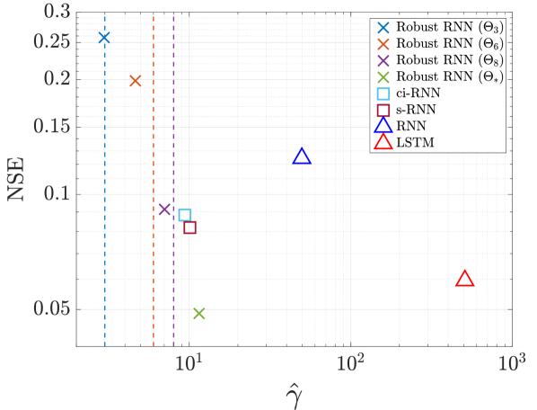
We have also plotted the worst case observed sensitivity versus median nominal test performance ( $\sigma_{u}=3$ ) in Fig. 5. The Robust RNNs show the best trade-off between nominal performance and robustness signified by the fact that they lie further in the lower left corner. For instance if we compare the LSTM with the Robust RNN ( $\Theta_{*}$ ), we observe similar nominal performance, however the Robust RNN has a much smaller Lipschitz constant. Varying the incremental $\ell_{2}$ gain allows us to trade off between model performance and robustness. We can also observe in the figure that the guaranteed upper bounds are quite tight to the observed lower bounds on the Lipschitz constant, especially for the set $\Theta_{3}$ .

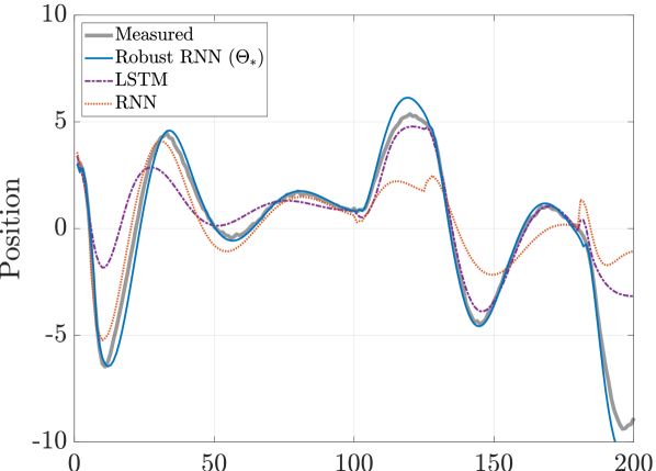
In Fig. 6, we have the model predictions for the RNN, LSTM and Robust RNN for a typical input with $\sigma_{u}=10$ . We can see that even with the larger inputs, the Robust RNN continuous to accurately track the measured data. The predictions of the LSTM and RNN however deviate significantly from measured data for significant periods.

References

[1] Y. Bengio, P. Simard, and P. Frasconi, “Learning long-term dependencies with gradient descent is difficult,” IEEE transactions on neural networks, vol. 5, no. 2, pp. 157–166, 1994.
[2] M. Cheng, J. Yi, P.-Y. Chen, H. Zhang, and C.-J. Hsieh, “Seq2sick: Evaluating the robustness of sequence-to-sequence models with adversarial examples.” in Association for the Advancement of Artificial Intelligence, 2020, pp. 3601–3608.
[3] G. Zames, “On the input-output stability of time-varying nonlinear feedback systems part one: Conditions derived using concepts of loop gain, conicity, and positivity,” IEEE Transactions on Automatic Control, vol. 11, no. 2, pp. 228–238, 1966.
[4] C. A. Desoer and M. Vidyasagar, Feedback systems: input-output properties. SIAM, 1975, vol. 55.
[5] W. Lohmiller and J.-J. E. Slotine, “On contraction analysis for non-linear systems,” Automatica, vol. 34, pp. 683–696, 1998.
[6] P. L. Bartlett, D. J. Foster, and M. J. Telgarsky, “Spectrally-normalized margin bounds for neural networks,” in Advances in Neural Information Processing Systems, 2017, pp. 6240–6249.
[7] S. Zhou and A. P. Schoellig, “An analysis of the expressiveness of deep neural network architectures based on their lipschitz constants,” arXiv preprint arXiv:1912.11511, 2019.
[8] T. Huster, C.-Y. J. Chiang, and R. Chadha, “Limitations of the lipschitz constant as a defense against adversarial examples,” in Joint European Conference on Machine Learning and Knowledge Discovery in Databases. Springer, 2018, pp. 16–29.
[9] H. Qian and M. N. Wegman, “L2-nonexpansive neural networks,” International Conference on Learning Representations (ICLR), 2019.
[10] S. L. Lacy and D. S. Bernstein, “Subspace identification with guaranteed stability using constrained optimization,” IEEE Transactions on automatic control, vol. 48, no. 7, pp. 1259–1263, 2003.
[11] D. N. Miller and R. A. De Callafon, “Subspace identification with eigenvalue constraints,” Automatica, vol. 49, no. 8, pp. 2468–2473, 2013.
[12] M. M. Tobenkin, I. R. Manchester, and A. Megretski, “Convex parameterizations and fidelity bounds for nonlinear identification and reduced-order modelling,” IEEE Transactions on Automatic Control, vol. 62, no. 7, pp. 3679–3686, 2017.
[13] J. Umlauft, A. Lederer, and S. Hirche, “Learning stable gaussian process state space models,” in 2017 American Control Conference (ACC). IEEE, 2017, pp. 1499–1504.
[14] J. Z. Kolter and G. Manek, “Learning stable deep dynamics models,” in Advances in Neural Information Processing Systems 32. Curran Associates, Inc., 2019, pp. 11 128–11 136.
[15] J. Miller and M. Hardt, “Stable recurrent models,” In Proceedings of International Conference on Learning Representations 2019, 2019.
[16] J. Umenberger, J. Wågberg, I. R. Manchester, and T. B. Schön, “Maximum likelihood identification of stable linear dynamical systems,” Automatica, vol. 96, pp. 280–292, 2018.
[17] M. Revay and I. R. Manchester, “Contracting implicit recurrent neural networks: Stable models with improved trainability,” Learning for Dynamics and Control (L4DC), 2020.
[18] J. Umenberger and I. R. Manchester, “Specialized interior-point algorithm for stable nonlinear system identification,” IEEE Transactions on Automatic Control, vol. 64, no. 6, pp. 2442–2456, 2018.
[19] E. Kaszkurewicz and A. Bhaya, Matrix Diagonal Stability in Systems and Computation. Birkhäuser Basel, 2000.
[20] N. E. Barabanov and D. V. Prokhorov, “Stability analysis of discrete-time recurrent neural networks,” IEEE Transactions on Neural Networks, vol. 13, no. 2, pp. 292–303, Mar. 2002.
[21] Y.-C. Chu and K. Glover, “Bounds of the induced norm and model reduction errors for systems with repeated scalar nonlinearities,” IEEE Transactions on Automatic Control, vol. 44, pp. 471–483, Mar. 1999.
[22] M. Fazlyab, A. Robey, H. Hassani, M. Morari, and G. Pappas, “Efficient and accurate estimation of lipschitz constants for deep neural networks,” in Advances in Neural Information Processing Systems, 2019, pp. 11 423–11 434.
[23] I. Goodfellow, Y. Bengio, and A. Courville, Deep learning. MIT press, 2016.
[24] J. L. Elman, “Finding structure in time,” Cognitive science, vol. 14, no. 2, pp. 179–211, 1990.
[25] A. Pinkus, “Approximation theory of the mlp model in neural networks,” Acta numerica, vol. 8, no. 1, pp. 143–195, 1999.
[26] S. Hochreiter and J. Schmidhuber, “Long Short-Term Memory,” Neural computation, vol. 9, pp. 1735–1780, 1997.
[27] D. P. Kingma and J. Ba, “Adam: A Method for Stochastic Optimization,” International Conference for Learning Representations (ICLR), Jan. 2017.

A Convex Parameterization of Robust Recurrent Neural Networks

Abstract

I INTRODUCTION

II Problem Formulation

Definition 1.

Definition 2.

III Robust RNNs

III-A Model Structure

III-B Description of Φ\Phi by Incremental Quadratic Constraints

III-C Convex Parametrization of Robust RNNs

Theorem 1.

Proof.

Theorem 2.

Proof.

Remark 1.

III-D Expressivity of the model set

Theorem 3.

Proof.

Remark 2.

Theorem 4.

Proof.

IV Numerical Example

IV-A Training Procedure

IV-B Model Evaluation

IV-C Results

References

III-B Description of $\Phi$ by Incremental Quadratic Constraints