A convex cover for closed unit curves has area at least 0.1
Abstract.
We improve a lower bound for the smallest area of convex covers for closed unit curves from to , which makes it substantially closer to the current best upper bound . We did this by considering the minimal area of convex hull of circle, line of length , and rectangle with side . By using geometric methods and the Box search algorithm, we proved that this area is at least . We give informal numerical evidence that the obtained lower bound is close to the limit of current techniques, and substantially new idea is required to go significantly beyond .
Key words and phrases:
Worm problem, Convex cover, Convex hull, Minimal-area cover, Closed curves1991 Mathematics Subject Classification:
Primary 52C15; Secondary 52A381. Introduction
Moser’s worm problem is one of many unsolved problems in geometry posed by Leo Moser [11] in 1966 (see [12] for a new version). It asked about the smallest area of region in the plane which can be rotated and translated to cover every unit arc. While this problem is still open, lower and upper bounds for this smallest area are available in the literature. The current best upper bound was established by Norwood and Poole [13]. For the lower bound, it is known only that the area of is strictly positive [10].
This problem can be modified by restricting region (e.g. triangle, rectangle, convex, non-convex, ect.) or restricting unit curves (e.g. closed, convex, ect.). Numerous problems in the worm family have been solved prior, see Wetzel [17] for a survey.
If we require to be convex, and cover arbitrary unit curves, the existence of the solution is shown by Laidecker and Poole [9] using Blachke Selection Theorem. In 2019, Panraksa and Wichiramala [14] showed that the Wetzel’s sector is a cover for unit arcs which has an area of . This cover is the current upper bound for this problem, whereas the current lower bound was found by Khandhawit, Sriswasdi and Pagonakis [8] in 2013.
The problem of finding smallest convex region to cover all (not necessarily unit) curves of diameter one was posed by Henri Lebesgue in 1914 and is known as Lebesgue’s universal covering problem. In this case, the current best lower and upper bounds are and due to Peter Brass and Mehrbod Sharifi [1] and Philip Gibbs [6], respectively.
In this paper, we consider the problem of covering closed unit curves by a convex region of the smallest area.
In 1957, H.G. Eggleton [3] showed that the equilateral triangle of side is the smallest triangle which can cover all unit closed curves and its area is . Twenty five years later, the smallest rectangle with lengths and is found by Shaer and Wetzel [15] and its area is about .
Furedi and Wetzel [5] decreased this area by clipping one corner of this rectangle with area about . Also, they modified this pentagon to a curvilinear hexagon which has an area of less than . In 2018, Wichiramala [18] showed that the opposite corner of the pentagon can be clipped to be a hexagonal cover with area less than which is the best currently known bound.
Our work focuses on a lower bound for this problem. Chakerian and Klamkin [2] applied Fáry and Rédei’s theorem [4] to find the first lower bound which is by considering the convex hull of circle and line segment in 1973. Further, Furedi and Wetzel [5] showed that the minimum area of convex hull of circle and the rectangle has area . Moreover, they replaced this rectangle by curvilinear rectangle and give a new lower bound about .
To improve this bound, one may consider the minimal convex hull of three given closed curves. However, in this case Fáry and Rédei’s theorem [4] can not be applied to find smallest area analytically, which complicates the analysis and call for the mix of geometric and numerical methods. Som-am [16] applied Brass grid method [1] to prove that the area of convex hull of circle, line segment ,and equilateral triangle is at least . In 2019, Grechuk and Som-am [7] used the Box search method to show that the minimal-area convex hull of the rectangle of perimeter , circle with perimeter , and the equilateral triangle with perimeter , is greater than . Thus, if we denote to be the area of smallest cover of closed unit curves, then
In this paper, we use geometric methods combined with the Box search algorithm to prove that the area of convex cover for the line segment, circle, and certain rectangle of perimeter is at least .
Theorem 1.1.
The area of convex cover for circle of perimeter , line of length , and rectangle of size is at least .
By Theorem 1.1, we have
which improves the previous bound . In fact, the true minimal area of in Theorem 1.1 is about , but we have rounded the bound to to simplify the proof.
The choice of line segment, circle, and rectangle in Theorem 1 was not an arbitrary or lucky one. In fact, we have used a systematic search for three shapes which gives the best possible lower bound.
The organization of this paper is as follows. A systematic search for three shapes which maximal possible area of minimal convex hull is presented in Section 2. The remaining sections are devoted to the proof of Theorem 1.1. Section 3 proves some geometric lemmas. Section 4 describes numerical box-search algorithm and computational results. The proof of Theorem 1.1 is finished in Section 5. We give some conclusions in Section 6.
2. A systematic search for shape
Theorem 1.1 establishes a new lower bound for the area of a convex cover for closed unit curves, by proving that a convex hull of three such curves, circle, line, and certain rectangle, must have area at least . In fact, the choice of these three curves was not an arbitrary or lucky one, but was the result of a systematic numerical search, which we will describe in this section.
This section contains neither proofs nor any form of rigorous analysis, and the reader who is interested only in the proof of Theorem 1.1 can go straight to the next sections. However, this section is important to understand how we selected three curves considered in Theorem 1.1, and provides some guide were to not look when trying to substantially improve our lower bound.
For each specific set of unit curves, we write a program which finds minimum area of a convex hull of these curves, where the minimum is taken with respect to all translations and rotations of the curves. We then modify the curves to make this minimal as large as possible. This result is a maximin problem with highly non-smooth and non-convex objective function. We used Matlab function, patternsearch, with random initial data to try to find the global optimal value in various cases.
Let be the area of smallest cover of closed unit curves. We will approximate curves by polygons, and it is clear that it suffices to consider convex polygons only. Let us start with 2 polygons. Let be the area of convex hull of polygons and . Let be the set of all orientation-preserving motions of the plane (that is, all possible compositions of rotations and translations). Then, given any two polygons and with unit perimeter, the solution of the minimization problem
| (2.1) |
is the lower bound for .
Now, our aim to find polygons and for which this lower bound is as large as possible. Let and be a number of vertices in polygons and respectively. We assume that and are fixed but and can vary. Let be the set of all convex polygons with vertices and unit perimeter. We consider optimization problem
| (2.2) |
It is clear that for any , ,
or, in words, is a lower bound for .
2.1. Numerical results for 2 objects
First, we construct a Matlab function NN2per to solve the minimization problem (2.1). The input of the function is coordinates of vertices of and . The function first calculates the perimeters of the polygons, and scale them to make the perimeters to be equal to . Then it applies the motion to , which is described by three parameters: vector of translation and angle of rotation , and use Matlab function convhull to estimate . We then use function MultiStart in Matlab to solve the minimization problem of the resulting convex hull area over parameters .
Second, we solve the maximization problem (2.2) by finding maximal possible output of function NN2per for fixed and . We start with some initial configuration (for example, is regular -gon and regular -gon), and then use the patternsearch function.
We repeat this procedure for various small values of and . Specifically, we consider the cases of a line and a triangle (2+3 points), two triangles (3+3 points), a triangle and a rectangle (3+4 points), two rectangles (4+4 points), and so on. The results are shown in Table 1.
| Type ( points) | Optimal area | Time (sec) |
|---|---|---|
| 2+3 | 0.072169 | 5889 |
| 3+3 | 0.072375 | 7995 |
| 3+4 | 0.085377 | 14080 |
| 4+4 | 0.085377 | 17370 |
| 3+5 | 0.087902 | 17296 |
| 5+5 | 0.087902 | 23684 |
| 9+19 | 0.095790 | 239828 |
| 20+20 | 0.096120 | 240258 |
| 9+50 | 0.096595 | 241172 |
| 11+50 | 0.096605 | 251041 |
From the Table 1, it can be seen that the maximum lower bound we found is , see Figure 1. This is close to the best known lower bound found from considering 2 objects [5]. We can conclude that in this case we did not improve the existing best lower bound but almost recovered the best result in the literature.

2.2. Numerical results for 3 objects
For three objects, we use the same idea as for 2 objects. Let be the third polygon with vertices which can be translated and rotated. We then solve the maximin optimization problem
| (2.3) |
where now denotes the area of convex hull of three polygons. Again, is the lower bound for .
For the internal minimization problem, we now optimize over six parameters which are and for translation and rotation of first and second polygons respectively. The maximization problem is now with respect to coordinates of polygon’s vertices.
We start the cases of line and two triangles (2+3+3), three triangles (3+3+3), two triangles and a rectangle (3+3+4) and so on. We can see the results in Table 2.
| Type ( points) | Optimal area | Time (sec) |
|---|---|---|
| 2+3+3 | 0.072169 | 25741 |
| 3+3+3 | 0.073086 | 29178 |
| 2+3+4 | 0.087867 | 35518 |
| 3+3+4 | 0.087887 | 38549 |
| 3+3+5 | 0.088478 | 51306 |
| 10+10+10 | 0.093546 | 208439 |
| 2+4+50 | 0.1004 | 327082 |
| 4+4+50 | 0.100403 | 505971 |
| 7+7+50 | 0.100417 | 1022268 |

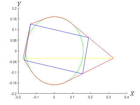
Table 2 shows that the maximum lower bound for we found is which is better than the current bound [7]. From the Figure 2, the three polygons corresponding to this lower bound approximates a circle of perimeter , a line of length and a rectangle of size .
Inspired by this result, we also try to find three objects in the form: circle, line, and -gon. We represent circle as regular -gon, line as a -gon, and then increased the number of vertices of the third polygon from to . The results are presented in Table 3.
Because -gon is a special case of -gon with coinciding vertices, the lower bound improves by definition, and it is best for . However, Figure 3 shows that the resulting -gon is very similar to the same rectangle of size which we have obtained in the experiment in Table 2. The resulting bound is also very close to the bound in Table 2.
| Type ( points) | Optimal area | Time (sec) |
|---|---|---|
| 3 | 0.0970429 | 13508 |
| 4 | 0.1003 | 28865 |
| 5 | 0.100304 | 33652 |
| 6 | 0.100374 | 54979 |
| 7 | 0.100386 | 80077 |
| 8 | 0.100390 | 81285 |
| 9 | 0.100418 | 119103 |
| 10 | 0.100473 | 123350 |
Based on the numerical experiments in this section, we
-
•
Have found a line-rectangle-circle configuration, whose convex hull is, numerically, always grater than . This significantly improves the previous best lower bound .
-
•
Conclude that no other “simple” configuration of 3 objects gives a substantially better bounds.
In the following section, we give a rigorous prove for the first conclusion, and this is the main result of this work. The second conclusion is informal and has no proof.
3. Geometric analysis
Let be a circle of perimeter , be a rectangle of size where and , and be line of length .
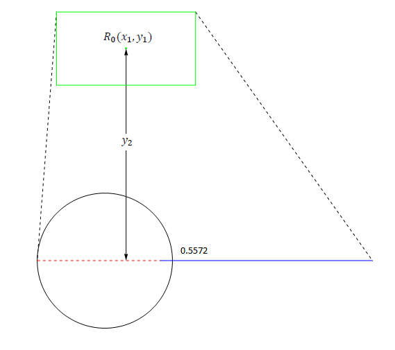
Let us fix the center of circle to be . Let be a regular -gon inscribed in , such that the sides of are parallel to some longest diagonals of . Let be a union . is called a configuration. Let be the convex hull of , and be the area of . Our aim is to find a configuration with the smallest .
Let be the center of . By the symmetry of circle, we may assume that . We have the vertices of are , , , and . Let be the center of and be the angle between X axis and , see Figure 4.

The vertices of are and . Note that any configuration is represented by , and . Clearly,
We define the function by mapping vector to . Clearly, is a continuous function. Since is a subset of , it suffices to show that
This would immediately imply Theorem 1.1.
Next, we will apply result of Fary and Redei [4], and Lemma 1 and Corollary 2 in [7] to bound parameters and .
Lemma 3.1.
Let be a region of points in satisfying the inequalities If for all , then in fact for all .
Proof.
Let be the area of convex hull of and only. By [4], is a convex function in both coordinates. By symmetry, . This combined with convexity implies that
whenever . Similarly,
whenever .
Let be the area of convex hull of and only. By [4], if moves in direction , attains minimum when is perpendicular to . Assume that or . Then .

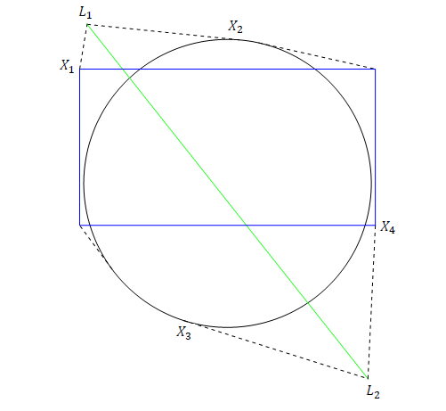
Let be the line segment between and . Next, let points be such that line segments and are perpendicular, see Figure 5. Then is trapezoid with bases lengths and , where . The area of is . Thus,
∎
Lemma 3.2.
Either , or is a subset of a rectangle with side lengths .
Proof.
By Lemma 3.1, we can assume that . Let and be the points of configuration with the lowest and highest -coordinates and , respectively. Because is below . Let be the height from to , respectively. if is below or on . Let . We have see Figure 6

Let and be the points of configuration with the lowest and highest -coordinates and , respectively. Let be any point in . If belongs to , then . Lemma 3.1 implies that if is any point on rectangle, then and if is any point on line, then . If , then . Otherwise, see Figure 7.

∎
We prove Lipschitz continuity of in in the following lemma
Lemma 3.3.
For every , and any , ,
with constants , , , , and .
Proof.
Let be a convex function on . If
then
see Lemma 5 in [7].

Hence,
Similarly, with for fixed ,
where and , see Figure 9, while with ,
where come from Lemma 3.2 and see Figure 10. Next, with ,
where ,


see Figure 10. This implies that
and
Finally, we need to prove that
| (3.1) |
To prove the bound for , we need the following claim.
Claim 1. The diameter of is less than .
By Lemma 3.1, the diameter is maximal possible if . Then . Let be a point which is maximum for all see Figure 12. By direct calculation, . Hence, the diameter of is .

Next, we will prove (3.1). We note that if (3.1) holds for , then it also holds for . Therefore it is sufficient to prove (3.1) only for sufficiently small .
Let with endpoints be the line rotated around by angle . Then . Similarly, .
By selecting sufficiently small, we can ensure that all vertices of polygons and coincides, except possible the endpoints of and . Then area difference is bounded by the total area of four triangles , , , , where are vertices by polygon adjacent to , see Figures 13 and 14.
Let be the height of triangle with respect to base . Let be the height of triangle with respect to base see Figure 14. By claim 1, We have .

∎
4. Computational results
Let be a region in Lemma 3.1. In this section, we prove that
by using box-search method as described in [7]. The method works as follows. Let be the center of a box which has the form . On every step, we check if
| (4.1) |
where is a half of the length of . If (4.1) holds, then inequality holds for every by Lemma 3.3.
If (4.1) does not hold, we will select the largest length, say and split into two boxes and . Then, if (4.1) holds for both boxes and , then holds for every and for every , hence it holds for every . If (4.1) does not hold for either or (or both), we subdivide the corresponding boxes again and proceed iteratively.
We start with , and, when the program halts, we are guaranteed that .
Let us illustrate the first step of this procedure. By Lemma 3.1, we start with . Then we check (4.1) for . In this case, (4.1) dose not hold because and . Thus, we must select the maximum length to subdivide into and . In this case, is the maximum. Hence, we divide into and . Then we check (4.1) for and for and repeat this procedure iteratively.
We run the Box-search algorithm [7] by using Matlab R2018a, see implementation details and Matlab code in Appendix. The programme halts after iterations. This rigorously proves that the minimal area is greater than . Numerically, the program returned value for this minimal area, with optimal configuration see Figure 15.
5. Main Theorems
Theorem 5.1.
(Theorem 1.1 in the Introduction) The area of convex cover for circle of perimeter , line of length , and rectangle of size is at least .
Proof.
Corollary 5.2.
Any convex cover for closed unit curves has area of at least .
Proof.
Let be a convex cover for closed unit curves. Then can accommodate , and , hence . Thus the area of is at least . However, by Theorem 1.1. ∎

6. Conclusion
In this work, we improve the lower bound for the area of convex covers for closed unit arcs from to . First, we used the geometric method to prove Lipschitz bounds for configuration function in parameters which represent the circle, rectangle, and line. Next, we used the numerical box-search algorithm developed in [7] to prove the main theorem. In fact, we have used regular -gon in place of circle for convenience of Matlab numerical computations.
The best bound we can in principle get from circle-line-rectangle configuration is . To improve beyond this, different configurations of objects should be considered. The numerical results in Section 2 suggest that no configuration of three objects can give a bound much better than this. Because considering and more objects significantly increases the number of parameters and is computationally difficult, it looks like bound (or slightly better) may be the limit of the current technique, and substantially new ideas are required to significantly improve it.
Appendix A Appendix
There are only two functions below which are used in Box-search method. First, function is used to find the area of convex hull for which are represented by . Second, function is used to check the main inequality (4.1) in a box domain by its parameters . Finally, the Box-search results is shown in A.3.
A.1. The box’s search results
| Percentage of | |
|---|---|
| 4.5964 % | 100000000 |
| 9.6894 % | 200000000 |
| 28.4273 % | 300000000 |
| 95.7067 % | 400000000 |
| 99.2349 % | 500000000 |
Table 16 shown the percentage of the area of the initial box for which the inequality (4.1) is verified and the iteration number every steps by Box search program.

Figure 17 illustrates the graphical process which ups to the number of iterations.
When the program finished, it displayed the result:
[r,n,min,xx1,yy1,xx2,yy2,app] = checkminNB5(0,0.0741,0,0.0976,-0.148,0.148,-0.148,0.148,0,pi,0.1,
0.0000001,0,0,0.11,0,0,0,0,0)
r = 0.001990679394226 (this is the area of the initial box, covered)
n = 527754566 (total number of iterations needed)
min = 0.100438196959697 (the minimal area convex hull)
xx1 = 0.004341796875000
yy1 = 0.006481250000000
xx2 = 0.004335937500000
yy2 = -0.004335937500000
app = 0.857111765231102 (the 5 coordinates for the optimal configuration)
References
- [1] Brass, P. and Sharifi, M., A lower bound for Lebesgue’s universal cover problem. Int. J. of Comp. Geom. & Appl. 15.05, 537–544 (2005).
- [2] Chakerian, G.D. and Klamkin, M.S., Minimal covers for closed curves. Math. Magazine. 46.02, 55–61 (1971).
- [3] Eggleston, H.G., Problems in Euclidean space: Application of convexity. Courier Corporation (2007).
- [4] Fáry, I. and Rédei, L., Der zentralsymmetrische Kern und die zentralsymmetrische Hülle von konvexen Körpern. Mathematische Annalen 122.03, 205–220 (1950).
- [5] Füredi, Z. and Wetzel, J., Covers for closed curves of length two Peri. Math. Hung. 63.01, 1–17 (2011).
- [6] Gibbs, P., An Upper Bound for Lebesgue’s Covering Problem. arXiv preprint math/0701393, (2018).
- [7] Grechuk, B. and Som-am, S., A convex cover for closed unit curves has area at least 0.0975 arXiv preprint math/1905.00333, (2019).
- [8] Khandhawit, T. and Pagonakis, D. and Sriswasdi, S., Lower bound for convex hull area and universal cover problems. Int. J. of Comp. Geom. & Appl. 23.03, 197–212 (2013).
- [9] Laidacker, M. and Poole, G., On the existence of minimal covers for families of closed bounded convex sets Unpublished, (1986).
- [10] Marstrand, J.M., Packing smooth curves in . Mathematika. 26.01, 1–12 (1979).
- [11] Moser, L., Poorly formulated unsolved problems of combinatorial geometry Mimeographed list, (1966).
- [12] Moser, W. OJ., Problems, problems, problems. Discrete Applied Mathematics. 31.02, 201–225 (1991).
- [13] Norwood, R. and Poole, G., An improved upper bound for Leo Moser’s worm problem Discrete and Computational Geometry. 29.03, 409-417 (2003).
- [14] Panraksa, C. and Wichiramala, W., Wetzel’s sector covers unit arcs. arXiv preprint arXiv:1907.07351, (2019).
- [15] Schaer, J. and Wetzel, J., Boxes for curves of constant length. Isr. J. of Math. 12.03, 257–265 (1972).
- [16] Som-am, S., An improved lower bound of areas of convex covers for closed unit arcs Master's thesis, Chulalongkorn University, (2010).
- [17] Wetzel, J.E., The classical worm problem—a status report. Geombinatorics. 15, 34–42 (2005).
- [18] Wichiramala, W., A smaller cover for closed unit curves Miskolc Mathematical Notes. 19.01, 691–698 (2018).