A Constraint on the Amount of Hydrogen from the CO Chemistry in Debris Disks
Abstract
The faint CO gases in debris disks are easily dissolved into C by UV irradiation, while CO can be reformed via reactions with hydrogen. The abundance ratio of C/CO could thus be a probe of the amount of hydrogen in the debris disks. We conduct radiative transfer calculations with chemical reactions for debris disks. For a typical dust-to-gas mass ratio of debris disks, CO formation proceeds without the involvement of H2 because a small amount of dust grains makes H2 formation inefficient. We find that the CO to C number density ratio depends on a combination of , where is the hydrogen nucleus number density, is the metallicity, and is the FUV flux normalized by the Habing flux. Using an analytic formula for the CO number density, we give constraints on the amount of hydrogen and metallicity for debris disks. CO formation is accelerated by excited H2 either when the dust-to-gas mass ratio is increased or the energy barrier of chemisorption of hydrogen on the dust surface is decreased. This acceleration of CO formation occurs only when the shielding effects of CO are insignificant. In shielded regions, the CO fractions are almost independent of the parameters of dust grains.
1 Introduction
Planets are believed to be formed in protoplanetary disks (PPDs) containing gas and dust. The dissipation timescale of PPDs, especially that of gaseous component, is of special importance for planetary system formation. The gas giant planets need to be formed prior to the significant dispersal of gas in disks (Mizuno et al., 1978; Tanigawa & Ikoma, 2007) and the gas dispersal may then lead to long term orbital instabilities of protoplanets that trigger their impacts (Iwasaki et al., 2001). The giant impacts between protoplanets are believed to form the terrestrial planets in the solar system.
Infrared emission from PPDs decreases in several million years (Haisch et al., 2001). Older faint disks around main-sequence stars are called debris disks (Hughes et al., 2018, for review), which might be explained by dust production due to collisional cascades starting from disruptive collisions of kilometer or larger bodies. That may be induced by planet formation events after gas dispersal such as giant impacts for terrestrial planet formation (e.g., Genda et al., 2015) or planetary accretion in outer disks (Kobayashi & Löhne, 2014). Sub-mm observations showed some debris disks with ages of several 10 Myrs still have molecular CO gas (Hughes et al., 2008; Dent et al., 2014; Moór et al., 2019). In the present work we aim to investigate if the gas in debris disks is a primary origin, i.e., the gas of PPDs is not fully dispersed, or secondary origin. This question is directly linked to how and when the disk gas dissipates.
In the secondary scenario, the observed CO is produced from solid bodies via collisions (Kral et al., 2016, 2017; Matrà et al., 2015, 2017, 2018). However, CO is photo-dissociated rapidly. For Pictoris whose disk has CO with , the dissociation timescale is about years so that the mass production of CO during the stellar age is estimated to be , where is the Earth mass (cf. Kral et al., 2016). The IR observations for comets by AKARI infer the fraction of CO to H2O (Ootsubo et al., 2012). Total solid bodies required for the observed gas is simply estimated from the CO mass and fraction to be , which is comparable to or larger than that of the solar system.
The gas production due to sublimation strongly depends on the temperature of parent bodies. Using the condensation temperature, the sublimation timescale is estimated to be 0.003 yrs for kilometer-sized CO bodies with 50 K, while it may be somehow longer for mixed ices. However, the timescale is much shorter than the ages of debris disks. It would thus be difficult to keep of CO in the icy bodies, unless there was a steady inflow from the outer colder regions. Carbon dioxide, CO2, can be another reservoir. CO observed around comets in our solar system is mainly explained by the photo-dissociation of CO2 (Weaver et al., 2011) so that CO might be less abundant than CO2 in comets. Outgassing CO2 changes into CO via photo-dissociation. Collisional vaporization occurs due to shock heating (Ahrens & O’Keefe, 1972; Kurosawa et al., 2010), so that high speed impacts ( km/s) are required even for vaporization of volatile materials (e.g., Okeefe & Ahrens, 1982; Kraus et al., 2011). The collisional velocities are estimated to be , where and are the orbital eccentricities and semimajor axes of colliding bodies, respectively, is the mass of the central star, and is the solar mass (e.g., Kobayashi & Löhne 2014). The collisional velocities of bodies with beyond 10 au are much slower than the vaporization velocity. The collisional outgassing of CO2 from cometary bodies is therefore difficult beyond 10 au, where CO gas is observed in debris disks. In summary, in the secondary-origin scenario, a large amount of reservoir ice is required, while it should be sublimated efficiently beyond au.
If the gas in debris disks is a primary origin, or is a mixture of primary and secondary components, CO can be reformed from C+ and C atoms in the gas phase. The required CO reservoir is then significantly reduced compared with the case of purely secondary gas. Higuchi et al. (2017) showed that the abundance ratio of atomic carbon to CO can be a probe of the abundance of H2 relative to carbon, i.e. the metallicity of gas in debris disks. If the gas is a remnant of PPDs , the metallicity is expected to be close to that of the interstellar medium (ISM). On the other hand, if gas is supplied from solid bodies, the metallicity is much larger than the ISM value while hydrogen is provided by H2O desorbed from solid bodies.
Although the CO chemistry in debris disks was investigated by many authors (Kamp & Bertoldi, 2000; Kamp et al., 2003; Gorti & Hollenbach, 2004; Hughes et al., 2008; Roberge et al., 2013), the elemental abundances in their models are not different from those in the ISM significantly. The metallicity can be different from the ISM value, depending on the origin of gas. Thus, in this paper, we examine how the CO chemistry depends on metallicity by calculating detailed chemical reactions and thermal processes, and the radiative transfer including exact line transfers in the debris disks.
This paper is organized as follows: one-dimensional plane-parallel PDR calculations. The results of the PDR calculations are described and an analytical formula for the amount of CO is developed on the basis of the plane-parallel PDR calculations in Section 3. Astrophysical implications are discussed in Section 4. Finally, our results are summarized in Section 5.
2 Methods and Models
2.1 Numerical Methods
The Meudon PDR code version 1.5.4 (http://pdr.obspm.fr/) is a publicly available photon dominated region (PDR) code which is designed to model a stationary plane-parallel slab of gas and dust controlled by far-ultraviolet (FUV) photons (Le Petit et al., 2006). A plane-parallel slab is illuminated by a radiation field penetrating from the left-side of the slab.
The Meudon code solves the radiative transfer at each point in the slab, taking into account dust extinction and line absorption of gaseous species. We use the exact method described in Goicoechea & Le Bourlot (2007) which allows us to take into account overlapping of the H, H2, and CO UV absorption lines. For the H2 line transfer, we define a value of under which the exact method is used. The FGK approximation proposed by Federman et al. (1979) is used for all electric transitions for , where is the lower level of Lyman and Werner transitions. We do not take into account the exact line transfer for 13CO and C18O.
Coupled with the radiative transfer, the full level population system of a number of species, including H2 and CO, is computed from the detailed balance between radiative transitions, collisional transitions, transitions due to the cosmic microwave background, formation and destruction processes both in the gas phase and on dust grains (Le Petit et al., 2006).
This treatment allows us to evaluate the H2 self-shielding effect more accurately than using the fitting formula provided by Draine & Bertoldi (1996), which has been used in most studies. Furthermore, the accurate calculation of the level populations provides the accurate rates of chemical reactions associated with excited H2, which will be discussed in Section 3.3. Similarly, the shielding effect of CO is calculated more accurately than using the table from Visser et al. (2009).
The Meudon code calculates the thermal equilibrium of gas and dust grains. For gas temperature, heating processes (including the photo-electric heating on dust, exothermic chemical reactions, and cosmic rays) are balanced with cooling processes (including infrared and millimeter emission from ions, atoms, and molecules). The treatment of dust grains is explained in Section 2.4. Chemical and thermal equilibria determine the abundances of each chemical species at each position.
In order to investigate the basic properties of the chemical structure of debris disks, in Section 3, we conduct simple plane-parallel PDR calculations of a semi-infinite gas slab with a uniform density illuminated by stellar radiation fields and the interstellar radiation field (ISRF).
We should note that the Meudon PDR code is not applicable directly to the multi-dimensional disk geometry because it is designed for the one-dimensional plane-parallel geometry. In debris disks, we should take into account the geometrical dilution of the stellar radiation and vertical ISRF. Nevertheless, we will find that the main underlying physics of debris disks can be approximated by the findings from the one-dimensional plane-parallel PDR calculations. In Section 4.2, we compare the observational results with the predictions obtained by applying the findings of the plane-parallel models to disk models.
2.2 Modifications to the Meudon Code
We made some modifications to the Meudon code because it is not designed for debris disks.
Firstly, we modified the calculation of the photo-dissociation of CO+. In calculating the photo-dissociation rate of species, the Meudon code divides the species into two groups. For one group, the photo-dissociation rate is estimated from a fitting formula, which is a form of , assuming the radiation field to be the ISRF (van Dishoeck et al., 2006), where is the fitting parameter. The rate is scaled by the ratio of the total UV flux to the ISRF flux. While this formulation is efficient and is often used in PDR calculations of debris disks, it can be inaccurate when the SED of the radiation field is different from the ISRF. In addition, the possible shielding of photo-cross sections that resonate with absorption lines is not considered in the exponential form. Since dust grains in debris disks are larger than those found in the ISM, is expected to be inaccurate.
For the other group, the photo-dissociation rate is computed directly from ; is the photo-dissociation cross section and is the radiation intensity summed over all incidence angles. This treatment allows us to evaluate the photo-dissociation consistent with the local radiation field at each position. It is however computationally expensive and used only for important species.
In the Meudon PDR code, CO+ was included in the former group where the fitting formula is used although CO+ is one of the most important species to form CO in debris disks. In this work, the photo-dissociation rate of CO+ is calculated from the numerical integration of , where is taken from Lavendy et al. (1993) (also see Heays et al., 2017), and tabulated as a function of the wavelength.
One of the important molecules to form CO in our results is the hydroxyl radical OH, whose photo-dissociation rate is computed directly from the integration of photo-reaction cross sections. It is dissociated by photons with wavelengths longer than 1100 Å. In the adopted radiation fields, the photo-dissociation rate of OH is mainly determined by the channel, which absorbs photons with Å(van Dishoeck & Dalgarno, 1983). We will define a normalized UV flux dissociating OH in Section 2.3.
Secondly, we modified the rate coefficient of an endothermic reaction of , which is one of the most important reactions to form CO. The Meudon PDR code treats endothermic reactions of C+, S+, O, and OH with H2, taking into account excited states of H2. Except for reactions of and 111 To estimate the enthothermic chemical reaction rates, the Meudon PDR code uses the results of the theoretical studies done by Zanchet et al. (2013b) and Herráez-Aguilar et al. (2014) for and by Zanchet et al. (2013a) for . the rate coefficients were calculated assuming that all the internal energies are used to overcome an activation barrier or an endothermicity. In order to calculate the reaction rate of more accurately, we use the fitting formulae for the rate coefficient of for , 1, 2, and 3 derived by Agúndez et al. (2010) based on the theoretical calculations by Sultanov & Balakrishnan (2005). The reaction rates for are replaced by that for , where is the vibrational quantum number. As a result, the total reaction rate may be underestimated. Recently, precise rates especially for have been estimated by Veselinova et al. (2021)222 O and H with does not affect the CO formation because the H fractions are too small to affect the CO formation. .
Thirdly, we do not consider heating owing to the di-electronic recombination. In the Meudon code, for simplicity, the electron captured in an upper electronic level is assumed to be de-exited only through collisions, resulting in gas heating. The density range considered in this paper is so low that most of transitions in the cascade of the captured electron will occur through spontaneous emissions. We only consider gas cooling owing to the removal of the kinetic energy of recombined electron.
2.3 Incident Radiation Fields
We consider two kinds of radiation fields which are incident on the edge of a semi-infinite gas slab.
One is the ISRF (Habing, 1968; Draine, 1978; Mathis et al., 1983). The ISRF is given by the summation of four components. One is the ISRF from far- to near-ultraviolet; an expression of the first component is given by
| (1) | |||||
for Å(Mathis et al., 1983)333Equation (1) is a fitting function of the results of (Mathis et al., 1983) as shown in the manual of the Meudon PDR code.. The second ISRF component is supplied by cold stars and is expressed as a combination of three black bodies at 6184, 6123, and 2539 K. The third component comes from the dust thermal emission which is estimated by the DustEM code (Compiègne et al., 2011). The forth ISRF component is the cosmic microwave background radiation given by a black body at 2.73 K.
The other radiation field is the stellar emission taken from ATLAS9 (Kurucz, 1992; Howarth, 2011). We consider two spectral types of A5V and A1V. The effective temperatures of the A5V and A1V stars are 8250 K and 9000 K, respectively. The metallicities of the stars are set to the solar value. The surface gravity is fixed to . Examples of the A5V and A1V stars are Pictoris (Lecavelier des Etangs et al., 2001) and 49 Ceti (Roberge et al., 2013), respectively.
As the stellar radiation incident into the slab, the radiation field at a representative distance of 50 au from the star is adopted. The mean intensities at au are shown in Figure 1.

We parameterize the UV fluxes that dissociate species which are important to form CO. The following two ranges of wavelengths are focused on.
One wavelength range is , which is shown by the gray region in Figure 1. The photons in this wavelength range photo-dissociate CO and H2, and photo-ionize C0. The FUV photon number flux integrated over the wavelength range is denoted by , and is often measured in units of the Habing (1968) field flux, cm-2 s-1 (Bertoldi & Draine, 1996). The normalized incident FUV photon number flux 444 In this paper, refers to an FUV field whose energy density at the surface of the gas slab is equal to that of the Habing field considering all steradian in the free-space. is given by
| (2) |
where indicates the normalized stellar FUV flux at a distance of 50 au from the central star, and is the normalized ISRF flux derived from Equation (1).
The other wavelength range is considered to characterize the OH photo-dissociation rate. The cross section of photo-dissociation of OH adopted in the Meudon PDR code has the two broad peaks centered around () and () (van Dishoeck & Dalgarno, 1983, 1984; Heays et al., 2017). The latter peak mainly contributes to the OH photo-dissociation while the contribution from the former peak is negligible. This is because as shown in Figure 1 the intensities of the stellar radiation increase rapidly with wavelength in the corresponding wavelength range. Considering that the intensities of the stellar radiation are an increasing function of wavelength within the latter peak, we set a wavelength range of , which corresponds to the long wavelength half of the latter peak. The OH photo-dissociation rate is roughly proportional to the FUV photon number flux integrated over this wavelength range, which is denoted by . For convenience, we use the normalized FUV flux .
From the stellar spectra of the A5V and A1V stars shown in Figure 1, one derives that are and , respectively. The contribution of the ISRF to is negligible, and for A5V and for A1V, respectively.
In this paper, the models with (, ) and those with ( and ) are referred to ”weak-FUV” and ”strong-FUV”, respectively.
2.4 Dust Properties
Dust grains play important roles in at least three processes. First, they are responsible for absorption and scattering of photons. Second, they work as a catalyst in some chemical reactions. For instance, H2 forms on the surface of dust grains rather than by gas phase reactions. Third, they contribute to thermal processes through photo-electric heating and collision with the gas. These processes depend significantly on the dust properties: the size distribution, dust-to-gas mass ratio, and chemical compositions.
2.4.1 Size Distribution
One of the differences of the debris disk from the ISM is absence of small dust grains. The small dust grains with radii smaller than m are blown out by the radiation pressure of stellar photons (Burns et al., 1979; Kobayashi et al., 2008, 2009). Absence of the small dust grains reduces the visual extinction, the H2 formation rate, and the photo-electric heating rate for a given dust-to-gas mass ratio. For simplicity, we consider spherical dust grains whose radii are denoted by . The power-law grain size distribution is assumed, where is the number density of the dust grains with the radius range from to (Mathis et al., 1977). This power-law size distribution is controlled by the collisional cascade (Dohnanyi, 1969; Tanaka et al., 1996), although the power-law index could be modulated due to the size dependence of collisional strength (Kobayashi & Tanaka, 2010). In this work, the minimum and maximum radii of the dust grains are fixed to m and m. We will discuss that our results do not depend directly on the size distribution in Section 3.1.
2.4.2 Composition
The dust grains are assumed to be a mixture of graphite and silicon. The absorption and scattering coefficients of dust grains are calculated by averaging those of the graphite and silicon in a ratio of , taking into account the size distribution. The heat capacity of the dust grains, which is used to determine the dust temperature at each dust size and position, is computed assuming the mixed composition. The absorption/scattering coefficients and heat capacity at each dust size are computed by Laor & Draine (1993) and Draine & Li (2001).
2.4.3 Charge of Dust Grains
In addition to the FUV flux, the charge of dust grains characterizes the photo-electric yield on the dust grain. The Meudon code takes into account the probability distribution function of the dust charge for each dust size , which is determined by collisional charging and photo-electric ionization (Bakes & Tielens, 1994), where is the dust charge.
As the grain size increases, the photo-electric ionization rate increases faster than the recombination rate. As a result, the charge of dust grains increases with . Since the maximum grain size considered in this work is up to 1 cm, a great number of the charge grid is required.
To reduce the computational cost, we approximate the charge distribution function at each grain size by a delta function of , where is the dust charge and is the mean charge for the grain size . The validity of the approximation is confirmed.
2.4.4 Dust-to-gas Mass Ratio
Since the dust-to-gas mass ratio of debris disks is unknown observationally and theoretically, a wide range of is considered in the present work. Using the size distribution , the dust-to-gas mass ratio is expressed as
| (3) |
where
| (4) |
is the total number density of dust grains, and are the mass and number density of element “x”, respectively, is the mean molecular weight per element “x” nucleus, and is the internal density of the dust grains. We should note that the gas mass density is expressed as because the gas component is considered on the basis of carbon. The gas metallicity is denoted by , and the elemental abundances of the gas phase used in the present work are shown in Table 1 for the solar metallicity . When changes, the relative abundances among metals are fixed. From Table 1, is given by
| (5) |
| atom | relative abundance of the gas phase | reference |
|---|---|---|
| He | ||
| C | 1 | |
| N | 2 | |
| O | 3 | |
| Ne | 4 | |
| Si | 5 | |
| S | 6 | |
| Ar | 7 | |
| Fe | 1 |
In the context of PPDs, is often determined from Equation (3) at a given . By contrast, we use the fact that in debris disks, the amount of dust grains is constrained by the optical depth at V band, which is often estimated from the fraction of the disk luminosity to stellar luminosity. The most practical criterion for debris disks is (Hughes et al., 2018), where denotes a typical vertical optical depth of debris disks. A typical optical depth along the mid-plane is given by , where is the aspect ratio of debris disks.
The mean free path of a photon for dust absorption depends on the grain size distribution as follows:
| (6) |
In the integration, the absorption coefficient can be set to be unity because is satisfied for m at the V band. Eliminating using Equations (3) and (6), one obtains
| (7) |
where is the mid-plane carbon nucleus column density of the gas phase at of the dust opacity at V band. The values of adopted in our PDR calculations will be shown in Section 2.5.
As mentioned in Section 2.4.1, the size distribution is used, and .
2.4.5 Temperature of Dust Grains
In the Meudon PDR code, the temperature of dust grains is computed from the energy balance between absorption of the radiation and thermal emission at each grain radius bin. For reference, we here show the grain temperature given by Hughes et al. (2008) as follows:
| (8) |
where is the stellar luminosity, is the grain radius, and is the distance from the central star. The dust temperatures obtained the PDR calculations are consistent with Equation (8).
2.4.6 Grain Surface Chemistry
The Meudon code takes into account H2 and HD formation with the Langmuir-Hinshelwood (LH) and the Eley-Rideal (ER) mechanisms (Le Bourlot et al., 2012). The grain-surface chemistry for other species heavier than H2 and HD is not included in this study because photo-desorption is so efficient that heavy species are difficult to freeze out on the grain surface (e.g., Grigorieva et al., 2007).
In debris disks, the most important H2 formation mechanism on dust grains is the ER mechanism involved by chemisorption of H atoms. This is because the dust temperatures, which are as high as 100 K as shown in Equation (8), are so high that a hydrogen atom physisorbed on the grain surface evaporates before it combines with another hydrogen atom.
In the ER mechanism, there are several free parameters in the Meudon PDR code. One is a sticking coefficient , which approaches zero for high temperatures because the hydrogen atom cannot stick on the dust grains owing to the excess kinetic energy. The Meudon PDR code adopts the empirical form , where K and are adopted (Le Bourlot et al., 2012).
Another parameter is corresponding to the energy barrier that a hydrogen atom overcomes to reach a chemisorption site on the grain surface. The H2 formation rate is highly sensitive to because the probability of overcoming the energy barrier is proportional to . Nonetheless, is highly uncertain. Its value depends on the surface condition and composition of dust grains. The energy barrier of chemisorption onto a perfect graphite surface is as high as K (e.g., Sha et al., 2002, by using quantum mechanics). This has been confirmed by the experimental study of a highly ordered pyrolytic graphite in the laboratory done by Zecho et al. (2002). By contrast, topological defects on the carbonaceous surface decrease , and can make chemisorption almost barrierless (K), depending on structures (Ivanovskaya et al., 2010). Experiments of chemisorption of H on porous, defective, aliphatic carbon surfaces have found that the activation energy is as low as K (Mennella, 2006). By contrast, in the cases with silicate, quantum chemical calculations revealed K both for crystalline silicate (Navarro-Ruiz et al., 2014) and amorphous silicate (Navarro-Ruiz et al., 2015), but they have not been confirmed experimentally yet.
Uncertainty of the H2 formation rate on warm dust grains also has been discussed in PDRs illuminated by strong radiation from massive stars. Except for the absence of small dust grains, the environments are similar to debris disks. In such PDRs, Habart et al. (2011) observationally found that rotationally-excited H2 is more abundant than the predictions of PDR models, suggesting that the H2 production rate on warm dust grains needs to be higher than a typical value (e.g, Jura, 1974). This result suggests that there is significant uncertainty in H2 formation rates on warm dust grains.
As will be mentioned in Section 2.5, considering the uncertainty of , is changed as one of the model parameters in our PDR calculations.
2.5 Model Parameters
We summarize the model parameters in our models and show their parameter spaces. The model parameters are divided into ones related to the radiation field, the dust, gas components, the H2 formation on the grain surface. The model parameters are tabulated in Table 2.
2.5.1 The Parameters Related to the Radiation Fields,
As mentioned in Section 2.3, in order to investigate how the CO chemistry depends on radiation fields, the weak-FUV and strong-FUV models are considered. They are characterized by and .
2.5.2 The Parameter Related to the Amount of Dust Grains,
The amount of dust grains is characterized by . We here estimate from observation results of Pictoris and 49 Ceti, which are examples of the stars having gas-poor and gas-rich debris disks, respectively. Since both the debris disks are almost edge-on, the observed column densities are comparable to those along the mid-plane. The total column density of species “A” integrated along the mid-plane is denoted by .
For Pictoris, several authors derive the C0 column densities from the [CI] - emission line (Higuchi et al., 2017; Cataldi et al., 2018) and absorption lines (Roberge et al., 2000). Their values range from to . The C+ column densities are estimated to be from the [CII] 158 m emission line (Cataldi et al., 2014, 2018) and absorption lines (Roberge et al., 2006). The CO column densities are estimated to be from emission lines (Higuchi et al., 2017) and from absorption lines (Roberge et al., 2000). These observations suggest that is comparable to , and is roughly two orders of magnitude smaller than and . The carbon nucleus column density is estimated to be . The spatial distribution of the dust surface area obtained by HST observations of Heap et al. (2000) is fitted by Fernández et al. (2006). The mid-plane optical depth is about , where the fitting formula is integrated over , which is the gas extent of the best fit model in Cataldi et al. (2018). Finally, is obtained for Pictoris.
For 49 Ceti, the C0 and CO column densities are estimated to be (Higuchi et al., 2019) and (Higuchi et al., 2020), respectively. The C+ column density is not well constrained because only a lower limit of the C+ mass, which is smaller than the CO mass, was obtained (Roberge et al., 2013). We however expect that is comparable to because should not be much larger than if all CO are formed through chemical reactions. The vertical optical depth estimated from the fractional luminosity is (Jura et al., 1993, 1998). Assuming that the aspect ratio of the dust distribution is , the mid-plane optical depth is . Finally, we obtain for 49 Ceti.
From and , a fiducial value of is set to (, ) because the behavior of the CO formation changes around for weak-FUV and strong-FUV as will be shown in Section 3.
In this paper, instead of , a normalized dust-to-gas mass ratio is used as the parameter indicating the amount of dust grains. Using Equation (7), one obtains
| (9) |
where is the dust-to-gas mass ratio at and given by
| (10) | |||||
where is used. We should note that although both and depend on and , the ratio is independent of the size distribution for a given .
To study how the amount of dust grains affects the thermal and chemical structures, the PDR calculations are performed with three different as listed in Table 2. For weak-FUV, since a typical is about for Pictoris, the cases with (, , ) are considered. For strong-FUV, since a typical is about , the cases with (, , ) are considered.
2.5.3 The Parameters Related to the Gas Component, ()
The parameters associated with the gas component are and metallicity . Given and , the corresponding hydrogen nucleus number density is , where is the carbon elemental abundance of the gas for (Table 1). The hydrogen gas density is difficult to constrain in most debris disks observationally although there are some successful exceptions which will be described in Section 4.4.
Fiducial carbon nucleus number densities are defined as for weak-FUV and for strong-FUV. The debris disk around Pictoris has a spatial extent of in the best-fit model in Cataldi et al. (2018, also see Section 4.2.2). A mean density is , which is comparable to the fiducial for weak-FUV. For 49 Ceti, because the radial extent is au, which corresponds to a cut-off radius of the surface density distribution (Hughes et al., 2018, also see Section 4.2.3), the mean density is , which is comparable to the fiducial for strong-FUV. For comparison, the densities 10 times larger than the typical are also considered for both the weak-FUV and strong-FUV models.
Next, we consider a range of the gas metallicity. The gas metallicity in debris disks depends on its origin. If the gas is a remnant of PPDs, the gas metallicity is expected not to be significantly different from the solar metallicity . It is maximized when all the gas comes from the secondary processes; hydrogen is provided by photo-dissociation of H2O outgassed from dust grains. In this case, the number of hydrogen nuclei becomes comparable to that of oxygen nuclei, and the gas metallicity reaches since at (Table 1). In this paper, a range of is considered.
2.5.4 The Parameter Related to the H2 Formation on the Grain Surface,
In order to investigate how the uncertainty of the H2 formation affects CO formation (Section 2.4.6), the cases with K and K are considered. The fiducial case K leads to a moderate H2 formation rate, corresponding to situations where chemisorption efficiently occurs on grains with plenty of surface defects (Le Bourlot et al., 2012). The cases with K give an upper limit of the H2 formation rate. Other parameters and are fixed to K and 1.5, respectively, because the gas temperatures do not exceed K in most cases.
| parameter | weak-FUV | strong-FUV |
|---|---|---|
| FUV flux (CO, H2, C+) | ||
| FUV flux (OH) | ||
| dust-to-gas mass ratio | , , | , , |
| gas density | ||
| the gas metallicity | ||
| [K](1) | 300, 10 | |
.
3 Results

3.1 Overall Behaviors of the Models with the Solar Metallicity
In this section, we investigate how the results of the fiducial models ( for weak-FUV and for strong-FUV) depend on the dust parameters and incident FUV fluxes (, ). The gas metallicity is set to .
We should note that the results with different and are not presented because our results are independent of both and as long as and remain unchanged. This is explained as follows. The grain-surface chemistry and photo-electric heating from dust grains are characterized by the total geometric cross section of dust grains . Equations (6) and (9) give
| (11) |
where we use the fact that because for m. Equation (11) shows that is controlled by and . Since is a given quantity, does not depend on the size distribution of dust grains if and are fixed. Thus, the thermal and chemical processes related to dust grains, i.e., H2 formation on dust grains and photo-electric heating, are independent of the size distribution for fixed and .
The results are shown in Figure 2. In this paper, instead of the optical depth, is used as a measure of the spatial coordinate, where is the carbon nucleus column density integrated from the slab edge to a given position. In Figure 2, the maximum column densities are set to for weak-FUV and for strong-FUV according to the observational constraints shown in Section 2.5.
3.1.1 Gas temperature
Figures 2a and 2b show that the gas temperatures increase with for both the weak-FUV and strong-FUV models because the photo-electric heating rate from dust grains, which is one of the dominant heating processes, increases in proportion to . A weak positive dependence of on is attributed to enhancement of the heating rate owing to the H2 formation on the grain surface.
3.1.2 Molecular Hydrogen
Before presenting the results, we introduce the analytic formation rate of H2 on grain surfaces,
| (12) |
(Le Bourlot et al., 2012), where Equation (11) is used, cm3 s-1 is a typical rate coefficient in the ISM (Jura, 1974), and is the chemisorption efficiency555 We should note that the Meudon code does not solve Equation (12) directly, but solves a set of rate equations considering chemisorbed hydrogen atoms and the dust size distribution (see Le Bourlot et al., 2012, for details). In addition to the chemisorbed H atoms, the Meudon code treats H2 formation with physisorbed H atoms. . Le Bourlot et al. (2012) derived
| (13) |
where and are defined in Section 2.4.6. For gas temperatures lower than K, which is satisfied in all the cases shown in Figure 2, the H2 formation rate is proportional to , and it depends sensitively on .
First, the cases with K are considered. Although H2 mainly forms on grain surfaces for the ISM, this may not be the case for debris disks because the H2 formation rate is extremely small. In order to examine the contribution of the grain-surface chemistry to H2 formation, we performed the additional PDR calculations where the grain-surface chemistry is switched off and plotted the results by the thin lines in the middle column of Figure 2. For (weak-FUV) and (strong-FUV), there are almost no changes in the H2 fractions with and without the grain-surface chemistry (Figures 2c and 2d), indicating that the grain-surface chemistry does not contribute to H2 formation. In this case, H2 is mainly formed in the gas phase, and the dominant chemical reaction is , where CH+ is formed by the radiative association between C+ and H666 Especially for metal-poor environments, the so-called H- channel is an important H2 formation path (e.g., Sternberg et al., 2021). Additional PDR calculations were performed with chemical reactions associated with H-, which had not been activated in the default setting of the Meudon code. The photo-detachment of H- is computed directly from (Section 2.2), where the cross section obtained in Wishart (1979) is used while the Meudon code calculates it by using a fitting formula. We confirmed that the H- channel does not affect the CO chemistry. .
The H2 formation rate of the grain-surface chemistry is enhanced in proportion to (Equation (12)) while the rate in the gas phase does not change. As shown in Figures 2c and 2d, is high enough for H2 to be formed mainly through the grain-surface chemistry when for weak-FUV and for strong-FUV.
For K, the H2 fractions stay low level even after they increase rapidly around owing to self-shielding (Draine & Bertoldi, 1996). This is because the H2 formation rate is so low that the destruction reactions in the gas phase and H2 photo-dissociation keep the H2 fractions low.
As mentioned in Section 2.4.6, there is large uncertainty in H2 formation on the warm dust grains with K. A decrease in from 300 K to 10 K significantly enhances the H2 fractions in Figures 2c and 2d because depends sensitively on . Considering the gas temperatures shown in Figures 2a and 2b, the H2 formation rate increases by a factor of at K and at K.
3.1.3 Carbon Monoxide, CO
First, the models with K are considered. Figures 2e and 2f show that does not depend on significantly as long as for both weak-FUV and strong-FUV. The CO fractions decrease with increasing because stronger FUV flux destroys CO more efficiently.
When is increased from to , the weak-FUV models show that the CO fractions increase by a factor of 2 or 3.
Acceleration of the CO formation owing to H2 is more significant for K than for K since a decrease in increases the H2 fraction (Section 3.1.2). The CO fractions monotonically increase with .
The -dependence of the CO fractions disappears when the grain-surface chemistry is omitted from the PDR calculations. This clearly indicates that the enhancement of the CO fraction for larger is related to efficient H2 formation on the grain surface.
How much H2 is needed to accelerate CO formation? Comparing between the middle and right columns of Figure 2, one can see that H2 fraction must be well above 0.1 for the CO fractions to increase by more than on order of magnitude. When the H2 fraction is comparable to 0.1 as in the strong-FUV models with (, K) and (, K), CO formation is not accelerated significantly.
In the deep interior , the CO fractions increase owing to shielding effects, which will be discussed in Section 3.2.3.
3.2 CO Formation in H2-poor Environments
In Section 3, we show that the CO formation is independent of the amount of H2 when H2 formation is inefficient in situations where is high and/or is small. In this section, we investigate how CO forms in such H2-poor environment, and develop an analytic formula for the CO fraction that is applicable in a wide range of in Sections 3.2.2 and 3.2.3.
3.2.1 Dependence of CO Fractions on Gas Metallicity
Figure 3 shows the spatial distributions of the CO fractions for various , , and listed in Table 2. The dust-to-gas mass ratios are fixed to for weak-FUV and for strong-FUV, where the CO formation proceeds, regardless of H2 (Figure 2).
We first focus on the CO fractions for . For given and the FUV fluxes (), the CO fractions decrease with increasing . Since is changed keeping constant, decreases with increasing . The CO fractions thus decrease with decreasing . This behavior has been pointed out by Higuchi et al. (2017); hydrogen is involved in CO formation.
Comparing between the panels of Figure 3, one can see that the CO fractions increase as increases and/or decreases. This behavior was qualitatively expected because the CO formation rate will increase with increasing and the CO destruction rate will decrease with decreasing .
For all the models shown in Figure 3, the CO fractions begin to increase in deep interiors owing to shielding effects, which will be investigated in Section 3.2.3.

3.2.2 An Analytical Formula for the CO Fraction
In this section, we develop an analytic formula for the CO fractions from the most important chemical reactions associated with CO formation of the H2-free gas in Figure 4. There are three main paths to form CO. At the high density limit (Equation (23)) , the CO formation is intermediated mainly by OH (PathOH). For lower densities, the dominant CO formation path depends on . At , the CO formation is intermediated by CH+ (Path). For higher , the CO formation proceeds without hydrogen as shown by the green arrows in Figure 4 (PathwoH).

The analytic formula taken into account all the chemical reactions shown in Figure 4 is complicated and is not useful. In Appendix A, we construct a fitting formula of the CO fraction based on PathOH, which is dominated for higher densities, as follows:
| (14) |
where
| (15) |
, is the relative oxygen abundance with respect to hydrogen in the gas phase, and corresponds to shown in Table 1.
3.2.3 Application of the Analytical Formula to Regions Where Shielding Effects Work
The analytic formula at a given position depends on , , and . Although and are given locally, is determined by the column densities integrated from sources of light. The FUV radiation that destroys CO can be attenuated by dust grains, C0, CO, and H2. In debris disks, the dust extinction is negligible.
Which of C0, CO, and H2 is more important for the shielding effects? In each shielding effect, one can define the critical column density at which is halved. Their critical densities are
| (16) | |||
is given by the results in van Dishoeck & Black (1988); we derive the H2 column density at which the shielding factor becomes 0.5 by the linear interpolation using Table 5 of their paper at (also see Visser et al., 2009). is given by , where is the cross section of photo-ionization of C0 (Heays et al., 2017), because the shielding factor owing to C0 is proportional to . is taken from the CO column density at which the shielding factor is 0.5 at in Table 5 of Visser et al. (2009, also see Equation (21)).
Let us estimate the importance of the shielding effect owing to H2. Considering the abundance ratio between hydrogen and carbon, one finds that the H2 column density is expressed as , where it is assumed that all hydrogen is in H2 () and all carbon is in C0 (). By contrast, in order for the shielding effect owing to H2 to be more important than the C0 attenuation, should be larger than , where the numerical factor corresponds to . This condition is not satisfied even for , and the shielding effect owing to H2 is not important compared with the C0 attenuation. For simplicity, the shielding by H2 is neglected in the analytic formula. We should note that the photo-dissociation rate may be overestimated in significantly shielded regions with .
In debris disks, C0 and CO contribute mainly to a decrease in . The problem is that the C0 and CO fractions both depend on local , which depends on their column densities. In this section, we construct a procedure to determine the the spatial distributions of , , and consistently.
Before presenting a way to evaluate the shielding effects, we should mention about the analytic formulae for and . The analytic formula for shown in Equation (14) is not applicable directly to a situation where carbon nuclei are mostly in CO because increases without limit as increases. To address this issue, Equation (14) is simply modified so that approaches smoothly in as follows:
| (17) |
This modification may be ad hoc, but it predicts the CO fractions consistent with those obtained from the PDR calculations as will be shown in Figure 3.
An analytic formula for the C0 fraction is presented. The C0 fraction is determined by the balance between photo-ionization of C0 and radiative recombination of C+ (Kamp & Bertoldi, 2000) as follows:
| (18) |
where the denominator guarantees that the sum of the C0, C+, and CO number densities is equal to , and is the ratio of the recombination to the ionization coefficients that is given by
| (19) | |||||
We confirmed that Equation (18) reproduced the C0 fractions obtained from the PDR calculations.
The normalized FUV flux is expressed in terms of the unattenuated value as follows:
| (20) |
where corresponds to the shielding factor, which depends on the C0 and CO column densities ( and ) computed from and , respectively. As the shielding factor, we adopt the following expression,
| (21) |
where the first factor on the right-hand side corresponds to the C0 attenuation, and the second factor is a fitting function of the self-shielding factor at tabulated in Visser et al. (2009).
The spatial distributions of , , and are determined consistently in a iterative manner by using Equations (17), (18), and (20).
It is useful to derive required to produce a specific value of the CO fraction. In the high density limit where PathOH is dominated, since the second term in the right-hand side of Equation (14) is negligible, Equation (14) is solved for as follows:
| (22) | |||||
which is valid when
| (23) |
Equation (22) is rewritten as
| (24) | |||||
which corresponds to the carbon nucleius density required to reproduce a specific value of . From Equation (24), an important conclusion can be drawn that decreases with increasing for fixed and . In other words, the upper limit of the CO fraction is obtained at .
3.2.4 Comparison of the CO Fractions with Those Predicted from the Analytical Formula
Figure 3 compares the results of the PDR calculations with the predictions from the analytic formula. reproduces the spatial profiles of reasonably well from the unattenuated regions () to the shielded regions () for all the parameter sets.
For lower shown in Figures 3a and 3c, the CO fractions begin to increase around , regardless of and . By contrast, Figures 3b and 3d show that the CO fractions with begin to increase at lower . This comes from the fact that CO self-shielding only works if the CO fraction is high enough; otherwise, C0 attenuation becomes more important.
A critical CO fraction above which CO self-shielding effect works is given by
| (25) |
The horizontal dashed lines in Figure 3 correspond to . In order to illustrate the effect of the CO self-shielding in Figure 3, we overplot the profiles of without considering the CO self-shielding effect in Equation (21) by the thick dashed lines. It is clearly seen that the CO self-shielding effect increases the CO fractions at only when exceeds .
The importance of C0 attenuation in CO formation has been pointed out by Kral et al. (2019).
3.3 Parameter Survey
In Section 3.2, we developed the analytic formula which reproduces the results of the PDR calculations reasonably well when the H2 fraction is too small to affect the CO formation. By contrast, in Section 3.1, we found that the models with lower and/or higher yield a sufficient amount of H2 to accelerate the CO formation. In this section, we investigate how the CO fractions depend on , , and for various , , and .

3.3.1 The CO Fractions at
First, we investigate the CO fractions at , which is the mid-plane column density inferred from the observational results of Pictoris (Section 2.5). At this column density, CO is not shielded by C0 attenuation significantly while CO self-shielding can work if the CO fraction is sufficiently high (Section 3.2.4). For reference, we also investigate the CO fractions at for strong-FUV. The top and middle panels of Figure 5 show the CO fractions as a function of for various , , and . Overall, as decreases and/or increases, the CO fractions increase and deviate from the predictions from the analytic formula.
First, we investigate the results with K (Figures 5a, 5c, 5e, and 5g). There is a critical () above which the CO formation is accelerated. depends on the parameters. For the fiducial weak-FUV models (), is around 1, regardless of (Figure 5a). For the high-density weak-FUV models (), depends on (Figure 5c). The models show acceleration of the CO formation at while is around 1 for .
The dependence of the CO fractions for the fiducial strong-FUV models () is similar to that for the high-density weak-FUV models () (see Figures 5c and 5e); enhancement of the CO fractions is seen only for when is increased from 0.1 to 1. For the high-density strong-FUV model (), for all .
The short summary is that for , for , and the models with show the intermediate behavior where takes values between 0.1 and 1 depending on . The dependence of on appears to be weak.

A decrease in reduces significantly. Figures 5b, 5d, 5f, and 5h show that for weak-FUV and for strong-FUV. The CO fractions monotonically increase with for most cases.
We should note that increases in the CO fractions appear to saturate for the weak-FUV models with (, , , K) and (, , , K). This is because the H2 fractions are close to unity in these models, and the enhancement of the H2 formation rate does not lead to further acceleration of the CO fractions.
The CO fractions at are affected by CO self-shielding when the CO fractions exceed (Equation (25)), which is shown by the horizontal dashed black lines. When , a small increase in for results in a large increase in at . This effect is clearly seen in Figures 5b and 5d.
What chemical reactions contribute to the acceleration of the CO formation? We found that vibrationally excited H2 (hereafter H) plays an important role. As a result, different reaction paths to CO are activated than the chemical reactions shown in Figure 4. It starts from which is known to be endothermic by K. The internal energy of H is available to overcome its energy barrier. The reaction between C+ and H with proceeds at almost the Langevin collision rate () (Hierl et al., 1997).
The efficiency of the mechanism is investigated in Zanchet et al. (2013b) and Herráez-Aguilar et al. (2014). In PDRs of the ISM, the importance of H was also pointed out in many references (Agúndez et al., 2010; Goicoechea et al., 2016; Joblin et al., 2018; Veselinova et al., 2021; Goicoechea & Roncero, 2022).
How much H is required to accelerate CO formation? Figure 6 shows the scatter plots of versus a boost factor , which is defined as the CO fraction divided by that at the H2-poor environments where only is changed to for weak-FUV and for strong-FUV, keeping the other parameters unchanged.
Figure 6 show that is correlated with for both weak-FUV and strong-FUV, indicating that H accelerates the CO formation. is larger than unity only when exceeds a critical H fraction of although there are large scatters.
The critical H fraction can be roughly understood as follows. A necessary condition affecting the CO formation by H is that the reaction rate of must be larger than that of . The condition becomes
| (26) | |||||
where is the reaction rate of . Figures 6 show that can distinguish whether to accelerate the CO formation or not.
The correlation between and depends on ; the models with lower tend to show larger at a fixed . This is because for smaller , the efficient formation of CH+ activates more reaction pathways involved by hydrogen to produce CO since increases with decreasing at a given .
3.3.2 The CO Fractions at
We investigate the CO fractions for strong-FUV at , which is the mid-plane column density inferred from the observational results of 49 Ceti (Section 2.5). At this column density, CO is shielded significantly.
Interestingly the CO fractions at show the opposite -dependence from that at . For K, increases in reduce the CO fractions (Figures 5i and 5k). The production of CH+ through the reaction between C+ and H does not contributes to the CO formation because the C0 attenuation makes the C+ fractions extremely low. That is why efficient formation of H2 no longer promotes the CO formation. Conversely, the presence of H2 negatively affects CO formation. In the chemical network shown in Figure 4, an increase in the amount of H2 reduces the amount of available H atoms, leading to a decrease in the CO formation rate.
A similar behavior is seen for K. As long as , increasing reduces the amount of CO. When is increased from to , the CO fractions turn to increase in Figures 5j and 5l. This is because most hydrogen exists as H2 for . The chemical reactions shown in Figure 4 no longer work, and different chemical reactions associated with H2 become important to form CO.
4 Discussion
4.1 Predictions of the Spatial Distributions of CO in a Disk Structure
The Meudon PDR code is not designed to investigate the chemical and thermal structure of disks. However, in Section 3.2, we developed the numerical procedure to determine the CO fractions on the basis of the findings of the plane-parallel PDR calculations. In this section, we present the method to derive the spatial distributions of and in a given disk structure using a similar method as shown in Section 3.2.3.

Figure 7 shows the disk structure considered in this paper. The disk extends from to , where the cylindrical coordinate is used and the central star locates at the origin. The density distribution of carbon nuclei is denoted as , and and are assumed to be uniform throughout the disk. At a certain position , the local radiation field is determined by the three rays, the stellar radiation that penetrates the disk from the inner edge to and the ISRF that propagates vertically from above and below the disk toward .
Applying Equation (20) into the cases with the disk geometry, one obtains as follows:
| (27) | |||||
where and are the normalized unattenuated FUV fluxes of the stellar radiation at a reference radius of and the ISRF, respectively. The geometrical dilution is considered in the first term on the right-hand side of Equation (27). A shielding factor is defined for each of the three rays; is the shielding factor of the stellar radiation, and () is the shielding factor of the ISRF coming from below (above) the disk. They are computed using Equation (21), but the column densities and are computed by integrating and along the corresponding rays, respectively.
The normalized FUV flux is given by
| (28) |
where is the normalized unattenuated FUV flux of the stellar radiation at . Shielding effects are not effective in as mentioned in Section 2.3
4.2 Comparison with Observations
Our analytical model shown in Section 4.1 is applied to the debris disks around Pictoris and 49 Ceti in Sections 4.2.2 and 4.2.3, respectively.
Although and are obtained throughout the disk, additional PDR calculations are conducted at various radii along the mid-plane considering the stellar radiation and vertical ISRF. There are two reasons for this. One is to verify whether and reproduce the results of the PDR calculations with K. The other is to investigate how the H2 formation accelerated by setting K affects the CO formation. Section 4.2.1 will describe how the PDR calculations are conducted taking into account the disk geometry.
4.2.1 PDR Calculations Using Disk Geometry and Structure
In the PDR calculation at , supposing that is the stellar radiation intensity and is the ISRF intensity, the mean intensity at is given by
| (29) | |||||
for Å, where is the geometrical dilution factor at , and we use the fact that . For the spectrum with Å, the shielding factors in Equation (29) are set to unity.
For each , we perform the PDR calculation with , , , and the radiation field shown in Equation (29). Since the geometrical dilution and shielding effects are already taken into account in the incident radiation, the chemical abundances at the optically thin limit () are considered as those at the position .
4.2.2 Pictoris
On the basis of the disk models shown in Cataldi et al. (2018), we here consider a ring with a uniform carbon nucleus vertical column density. With the C0 and C+ line data (Cataldi et al., 2014, 2018), Cataldi et al. (2018) derive the best fit parameters of and au. The stellar parameters of the central star adopted here are the same as those of the A5V star shown in Section 2.3. The scale height is , where is the sound speed with the constant temperature and .
Since for Pictoris (Section 2.5), an average mid-plane carbon nucleus number density is estimated to be . In order to investigate how the CO fractions depend on the mid-plane density, we consider two different values of at the inner edge, (low-density model) and (high-density model) as listed in Table 3.
| low-density | high-density | |
| [](1) | 75 | 190 |
| [](2) | ||
| [](3) | ||
| 5.0 | 2.0 |
The radial distribution of the mid-plane density is given by
| (30) |
where the mean molecular weight is assumed to be spatially constant.
The mid-plane column densities integrated from to for both the models are shown in Table 3. They correspond to the minimum and maximum values of the observed C0 column densities multiplied by two (Higuchi et al., 2017; Cataldi et al., 2018), where the factor two comes from the contribution from C+.
The vertical column density is determined by multiplying by the scale height, which depends on and . Although depends on the chemical state of the species, for simplicity, we assume that all gases are neutral atoms, and is given by . Even when the gas is fully molecular, our results do not change significantly because will be about a factor of two larger and the vertical column density decreases by about 30%.
Referring to Equation (9), the dust-to-gas mass ratio is expressed in terms of and as follows:
| (31) |
From Equation (31), the dust-to-gas mass ratios are given by for the low-density model and for the high-density model, where is used (Table 3).
Using the analytical model presented in Section 4.1, the spatial distribution of is obtained. Figures 8a and 8b show at the mid-plane as a fuction of . is almost constant because the ISRF gives dominant contribution in most radii except near the inner edge. Since the vertical column density for the high-density model is around , is slightly attenuated. By contrast, at the mid-plane decreases with owing to the geometrical dilution.
Before showing the results of the PDR calculations, we present the approximate formula of the predictions from the analytic formula. Equation (23) can be rewritten as . Since and , Equation (24) is valid for . Equating the mid-plane density and the density required to produce a given CO fraction (Equation (24)), the CO fraction is expected to be
| (32) | |||||
where Equation (28) is used for , and is the attenuated local value. Integrating over the disk extent with Equations (30) and (32), one obtains the predicted mid-plane CO column density,
| (33) | |||||
where is the average of weighted by over the disk extent.
The PDR calculations are conducted at four radii, au, au, 100 au, and 120 au.

Firstly, the cases with are considered. The results of the PDR calculations of the low-density and high-density models are shown in Figures 8c and 8d, respectively. For K, the radial profiles of are consistent with the predictions from the analytic model (Section 4.1) for both the models because H2 formation is inefficient. Although is slightly larger than unity, the effect of excited H2 is limited as shown in Figure 5a.
When is decreased from K to K, the H2 formation rate increases by about four orders of magnitude at K, making a large amount of hydrogen nuclei being molecular. As a result, H increases the CO fraction by about an order of magnitude in both the models (Figures 8c and 8d). This is consistent with what we found in Figure 5b.
The mid-plane column densities of C0 and CO integrated from to are shown in Figures 8e and 8f as a function of . After a rapid increase in near the inner edge, they become almost constant outside from au. This clearly shows that the CO mid-plane column densities are determined near the inner edge, and CO in the outer disk does not contribute to the total column density.
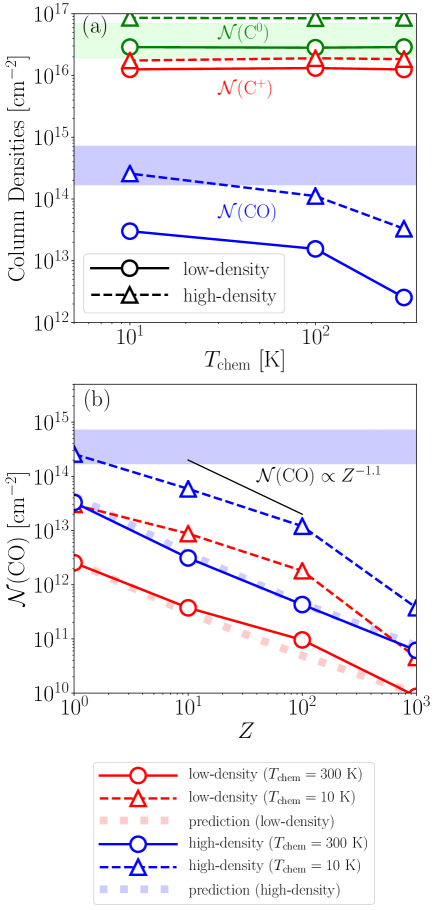
In order to compare our results with the observational results, the mid-plane column densities of C+, C0, and CO integrated from to are shown as a function of in Figure 9a. The C0 column densities of the low- and high-density models are both consistent with the observational results, and do not depend on .
The CO column densities increase as the mid-plane gas density increases and/or decreases. The high-density models produce about an order of magnitude larger CO column densities than the low-density model for all . This comes from the fact that (Equation (33)). The contribution of the attenuation of to an increase in is limited since the vertical column density is comparable to or smaller than (Table 3). The CO column density of the high-density model with K does not reach the lower limit of the observational constraints (Higuchi et al., 2017). If is lower than 100 K, the high-density models yield the CO column density comparable to the observational constraints.
The dependence of is shown in Figure 9b. For the fiducial models ( K), decreases with increasing , roughly following the predictions from Equation (33). When decreases to K, is increased by an order of magnitude, keeping the dependence almost unchanged (also see Figure 5b). Figure 9b shows that metallicities larger than cannot reproduce the observational CO column densities even when the H2 formation is enhanced by decreasing .
4.2.3 49 Ceti
Following Hughes et al. (2017) and Higuchi et al. (2019), we adopt the disk model which has a power-law distribution with the inner edge at and with a exponential cut-off at ,
| (34) |
where au, , and au are the best fit parameters. The outer edge of the disk is at infinity. The scale height is , where is the sound speed with and , where is the central star mass (Hughes et al., 2018, also see Table 5).
As discussed in Section 2.5, a typical mid-plane number density of carbon nuclei is given by , where is divided by the disk extent . We consider two different values of the mid-plane carbon nucleus density at , (low-density model) and (high-density model).
| low-density | high-density | |
| [](1) | ||
| [](2) | ||
| [](3) | ||
| 0.24 | 0.06 |
The mid-plane density is given by
| (35) | |||||
where is assumed to be spatially constant. The corresponding mid-plane column densities are listed in Table 4. The high-density model gives the mid-plane column density comparable to or slightly larger than that predicted in Higuchi et al. (2019). As in the case of Pictoris, the vertical column densities are determined by assuming all the gas is neutral atomic, and the values with at au are listed in Table 4.
Substituting into Equation (31) gives for the low-density models and for the high-density models, where is used. Since is much lower than unity, the acceleration of the CO formation owing to H is not effective (Section 3.3.1).
| SSUV | WSUV | |
|---|---|---|
Different stellar parameters are used in the literature (Chen et al., 2006; Hughes et al., 2008; Montesinos et al., 2009; Roberge et al., 2013). Among the different stellar models, the two extreme stellar models that provide the smallest and largest are considered. The stellar parameters of these models are summarized in Table 5. The strong and weak stellar UV models are called SSUV and WSUV, respectively.

Equating Equations (35) and Equation (24), one obtains the expected CO fraction,
| (36) | |||||
where shows of the SSUV model.
Models SSUV (WSUV) with the lower and higher mid-plane densities are called SSUVlow (WSUVlow) and SSUVhigh (WSUVhigh), respectively.
First, the low-density models are focused on. Figures 10a and 10b show the radial distributions of the normalized UV fluxes for models WSUVlow and SSUVlow, respectively. Since the C0 fractions are smaller for SSUV owing to the stronger FUV flux, decreases more slowly for SSUVlow than for WSUVlow. As a result, more outer parts of the disk is exposed to intense FUV radiation for SSUVlow. The FUV fluxes take minimum values in au for WUVlow and in au for SUVlow, and then increases to around au. For WSUVlow, the vertical attenuation of is clearly seen in au because is larger than (Table 4).
The radial profiles of the C0 and CO fractions in the low-density models with are shown in Figures 10e and 10f. For K, both the models clearly show that CO forms efficiently only in the region where the stellar radiation flux is low because is in proportion to . Their radial distributions agree with the predictions from the analytic model (Section 4.1).
A decrease in does not affect the CO fractions significantly, compared with the results with Pictoris (Figures 10e and 10f). The CO fractions are increased only by a factor of 2 or 3. This comes from the fact that for 49 Ceti is more than one order of magnitude smaller than that for Pictoris. Roughly speaking, the inner (outer) regions dominated by the stellar radiation (the vertical ISRF) correspond to the strong-FUV (weak-FUV) models at . As seen in the first and middle panels of Figure 5, when , the existence of H increases the CO fractions only by a factor of 2 or 3.
When the mid-plane density increases, the behaviors of the CO fractions change significantly. The stellar radiation in the wavelength range of is almost attenuated in very inner regions even for model SSUVhigh. Since the vertical column density at au (Table 4) is much larger than , the vertical attenuation of the ISRF is significant in (Figures 10c and 10d).
Figures 10g and 10h show that both the high-density models yield large amounts of CO where is almost attenuated. The CO fractions in the attenuated regions are almost independent of . This is consistent with the results shown in Section 3.3.2. In a such attenuated region, does not accelerate the CO formation because of depletion of C+. We should note that the CO fractions slightly decrease with decreasing in the attenuated regions because the H atoms available for the CO chemistry shown in Figure 4 are reduced by enhancement of the H2 formation (Section 3.3.2)
The bottom panels of Figures 10 show the radial distributions of and integrated from the inner edge to . Increases in the CO column densities are saturated around the peak radius of . Thus, is determined in the amount of CO inside the peak radius of .

The obtained C+, C0, and CO column densities integrated along the mid-plane are compared with the observational results in Figure 11a for . The low-density models show that the CO fractions does not reach the observed values for both the stellar models. By contrast, the high-density models produce sufficient amounts of CO to explain the observational results. We thus expect that there is a best solution to explain the observed CO column densities in (Table 4). For reference, we conducted additional PDR calculations with (). The mid-plane density is between those in the low-density and high-density models. Figure 11a show that a best solution is located in , and both and of a best solution will be consistent with the observational results.
The dependence of is shown in Figure 11b. For all the models, the CO column densities decrease with increasing as , and are consistent with the predictions from Equation (36). Figure 11b shows that WSUVhigh (SSUVhigh) provides consistent with the observed CO column densities if (). This suggests that if the gas is secondary-origin (), the CO column densities cannot be explained only by steady-state chemical reactions.
4.3 Uncertainty of the H2 Formation on Dust Grains
One of the main results of this paper is that the CO formation is affected strongly by , which is one of the uncertain parameters in the ER mechanism, when the shielding effects are not significant. In this section, other uncertainties of the H2 formation are discussed.
Another factor not considered in this paper is stochastic effects. Fluctuations of the number of H atoms on the grain surface should be take into account when few reactive H atoms are on the grain surface (Le Petit et al., 2009). We confirmed that the number density of the H atoms physisorbed on the grain surface is much smaller than the number density of dust grains. This indicates that the master equation should be used instead of the rate equation to accurately estimate the H2 formation rate of the LH mechanism. Bron et al. (2014) found that the LH mechanism becomes an efficient H2 formation mechanism in unshielded PDR regions even when the dust temperature is high for the interstellar environment. It is still unknown how the fluctuations of the number of physisorbed H atoms affect H2 formation in debris disks.
Fluctuations of the dust temperature also affects the H2 formation for small grains with m (Cuppen et al., 2006). If only large dust grains exist in debris disks, dust temperature fluctuations are negligible because of their large heat capacities. If small dust grains exist in debris disks, their temperature fluctuations may affect the H2 formation rate.
4.4 Caveats
Our analytic formula of enables us to predict the CO spatial distributions at a given and stellar radiation field (Section 4.1). Comparison of our results with observational results gives a constraint on the gas metallicity. In order to confirm whether the steady-state chemistry is a promising mechanism to produce the observed amount of CO, it is crucial to constrain the gas metallicity by other methods.
We should note that the column density of hydrogen is constrained by several observations for the debris disk around Pictoris. Freudling et al. (1995) obtained an upper limit of the HI column density, from non-detection of the 21 cm line. Lecavelier des Etangs et al. (2001) found that the H2 column density should be smaller than because H2 absorption lines are not detected. Using a C0 column density of cm-2 (Higuchi et al., 2017), is estimated to be larger than , which is much larger than . Recently Matrà et al. (2017) constrained the hydrogen number density by the line ratio of CO () and CO (); their result suggests that should be smaller than . If this is the case, the observed CO fractions may not be explained by such a small value of even if is sufficiently low. The combination of our results and the observational constraints may rule out the primordial origin () of the gas in Pictoris.
Although we found that there is a parameter set which may explain the amount of CO by considering only steady-state chemical reactions in Sections 4.2.2 and 4.2.3, we need to compare our models with observational results in more detail by performing synthetic observations of our disk models.
For 49 Ceti, Higuchi et al. (2020) showed that the excitation temperatures need to be as low as K by conducting non-LTE analysis of the rotational spectral lines of CO considering isotopologues line ratios (also see Kóspál et al., 2013). In our PDR calculations of 49 Ceti, the gas temperatures do not fall below K. This low excitation temperature may suggest that level populations are not thermalized because of low .
We will address direct comparisons between the chemical model and observational results in forthcoming papers.
4.5 Dissipation of Protoplanetary Disks
If the gas in debris disks contains a significant amount of H2, the gas of PPDs still remains, at least partially, in debris disks; i.e. the timescale of PPD gas dispersal is longer than the age of debris disks. Many authors investigated the gas dispersal of PPDs through magnetically-driven winds (Suzuki & Inutsuka, 2009, 2014) or/and photo-evaporation by UV/X-rays (Hollenbach et al., 1994; Gorti & Hollenbach, 2009; Owen et al., 2012; Nakatani et al., 2018). EUV photo-evaporation (Hollenbach et al., 1994) is expected to be inefficient in debris disks around A-type stars because they emit less EUV than either lower and higher mass stars. FUV photo-evaporation would be important at large radii au as long as a large amount of small dust grains exist (Gorti & Hollenbach, 2009). During the evolution from a PPD to a debris disk, an amount of dust grains decreases and the grain size increases. Nakatani et al. (2021) recently found that this evolution of dust grains suppress photo-electric heating, making FUV photo-evaporation ineffective. As a result, the lifetime of the gas component is determined by EUV photo-evaporation. Suppose that the EUV flux of an A type star is about , the photo-evaporation is at least (Gorti et al., 2009). If the initial disk mass at the point small grains have been depleted is , the lifetime is about Myr, indicating that the lifetime can be longer than Myr. However, the EUV flux in young A-type stars is highly uncertain, and how protoplanetary disks evolve into small-grain-depleted disks are unknown. Further investigations are needed. The future high resolution observation for the ratio combined with Equation (14) would give the distribution of in depleting PPDs, which may reveal the physics of disk dispersal.
5 Summary
In this paper, we investigated the CO chemistry in optically thin PDRs with larger dust grains than the ISM as a model of debris disks. Because hydrogen is involved in CO formation, the CO abundance should depend on the hydrogen density. This may allow us to constrain the amount of hydrogen if we know how much carbon nuclei becomes CO (Higuchi et al., 2017).
We investigated CO formation only through steady chemical reactions without considering any secondary processes. For simplicity, we consider a stationary plane-parallel semi-infinite uniform slab which is illuminated by the interstellar standard radiation and stellar radiation from its edge. We compute the chemical and thermal equilibria taking into account detailed radiative transfer using the Meudon PDR code (Le Petit et al., 2006; Goicoechea & Le Bourlot, 2007; Le Bourlot et al., 2012). Although the plane-parallel geometry is far from the disk geometry, we found that the chemical structure of debris disks can be approximated by the findings from the one-dimensional plane-parallel PDR calculations.
The model parameters are the carbon nucleus density , gas metallicity , FUV photon number flux that dissociates CO normalized by the Habing flux, the dust-to-gas mass ratio , and , which corresponds to the energy barrier of chemisorption. The model parameters are tabulated in Table 2. We call the models with weaker and strong FUV incident fluxes ”weak-FUV” and ”strong-FUV”, respectively. The dust-to-gas mass ratio is expressed in terms of the carbon nucleus column density at (), where is the mid-plane optical depth (Equation (7)). Observations of debris disks can constrain . As a fiducial value of , is adopted. The corresponding dust cross section is 80 times smaller than that in the ISM. A fiducial dust-to-gas mass ratio is defined as at . The ratio is equal to , and determines the dust surface area (Equation (11)). Considering large uncertainty in H2 formation on the grain surface, we explore a range of H2 formation rates on dust grains with a dust temperature of K by adopting K and 10 K. The K case gives an upper limit of the H2 formation rate since there is almost no energy barrier in chemisorption.
Our results are summarized as follows:
-
1.
For higher and smaller , we found that CO formation proceeds in the H2-poor environments without the influence of H2. Our environments tend to have a very low H2 abundance because the low grain surface area, high dust temperatures, and low gas temperatures make H2 formation extremely inefficient if the activation barrier is as high as K. We developed an analytical formula for the CO fractions (Section 3.2). The analytic formula is applicable even in shielded regions by using the local flux attenuated by C0 and CO, and reproduces the spatial distributions of the CO fractions obtained from the PDR calculations reasonably well (Figure 3).
-
2.
From the high density limit of the analytic formula for (Equation (14)), we obtain the hydrogen nucleus number density required to produce a given as a function of the FUV flux and gas metallicity (Equation (22)). If the amount of carbon nuclei and local FUV flux are fixed, lower metallicity produces a larger amount of CO because there are more H atoms to start the chemistry that produces CO.
-
3.
The H2 formation rate depends sensitively on since it is proportional to . The smaller , the more active the H2 formation on the grain surface. Increases in also enhances the H2 formation. The CO formation is accelerated by vibrationally-excited H2, whose internal energy is used to overcome an endothermicity of . The enhancement of the CO fractions owing to the excited H2 is occurred only when the shielding effects are insignificant. If the shielding effects are important, the CO fractions show different dependence on and . As decreases and/or increases, the CO fractions decrease although the dependence is weak. This is because in such a shielded region, the C+ fractions is too low for to accelerate the CO formation. A decrease in the number of H atoms available for CO formation decreases the CO fractions.
-
4.
A critical dust-to-gas mass ratio above which the CO formation is accelerated depends sensitively on . For K, roughly speaking, is about although it depends on and (Section 3.3). A decrease of from 300 K to 10 K reduces significantly; for weak-FUV and for strong-FUV.
-
5.
CO is self-shielded but also shielded by C0. Which shielding effect of CO is effective depends on at the low limit (Section 3.2.3). For at , CO is self-shielded for . When the CO fraction is sufficiently smaller than , the C0 attenuation increases the CO fraction for before CO self-shielding becomes important.
- 6.
The chemical structure of debris disks have not been studied by taking into account detailed chemical processes consistent with radiation transfer. Particularly, it may be important to consider level populations of H2 accurately because for lower and/or higher excited H2 can promote endothermic formation reactions of CH+ to accelerate the CO formation.
In this paper, an interstellar C/O ratio of 0.4 is used (Table 1). Recently Kama et al. (2016) and Bergin et al. (2016) however found evidence that C/O ratios could exceed unity in PPDs, indicating that C/O ratios change from the interstellar value during the evolution of PPDs. If a part of the gas in a debris disk comes from a remnant PPD, the C/O ratio could exceed unity also in a debris disk. From our analytic formula for the CO fraction (Equation (14)), it is expected that the CO fraction changes in proportion to .
Our results were compared with the observational results of the debris disks around Pictoris and 49 Ceti in Sections 4.2.2 and 4.2.3, respectively.
For Pictoris as an example of gas-depleted debris disks, the steady chemical model is difficult to produce a sufficient amount of CO to fit the observational results if the fiducial parameter K of the Eley-Rideal mechanism for the formation of H2 on warm dust grains is adopted. The higher the metallicity, the more inefficient CO formation becomes, due to the lack of H atoms to facilitate its formation. The CO column densities decrease as . If is lower than 100 K, the steady chemical model may explain the observed amount of CO due to the H2-accelerated CO formation only if (Figure 9). If , the steady chemical model cannot produce a sufficient amount of CO even when the H2 formation on dust surfaces are efficient.
For 49 Ceti as an example of gas-rich debris disks, the CO fraction is sensitive to the column density of carbon nuclei (Figure 11). Our results show that there is a solution that may explain both the observed CO and C0 column densities (Higuchi et al., 2020) in a reasonable range of for (Higuchi et al., 2019). Since the dust-to-gas mass ratio is extremely small and shielding effects are significant, the CO fraction is insensitive to . As in the case of Pictoris, the observed CO column density cannot be reproduced for 49 Ceti if .
We should note that steady state chemical models can explain Pictoris and 49 Ceti only under a very restricted set of parameters, including enhanced production of H2 on grains and . However, for Pictoris, complementary published observations mentioned in Section 4.4 indicated much lower H or H2 densities than are required. The combination of this work and the constraints on the H and H2 reveals that steady state chemistry cannot explain the observations.
As mentioned in Section 1, if the gas in Pictoris is secondary-origin and CO is supplied from solid bodies through collisions, a required injection rate of CO is estimated by the observed CO mass divided by the CO photo-dissociation timescale. Our results clearly show that the CO formation rate with is too small to explain the observed amount of CO. The total solid bodies required to provide CO during the stellar age is about taking into account an expected fraction of CO in the solid bodies (also see Dent et al., 2014). As pointed out in Section 1, we need to consider detailed outgassing processes from solid bodies in order to investigate if the required amount of CO can be supplied. In addition, the gas should be removed at a timescale comparable to the CO photo-dissociation timescale because C0 and C+ are accumulated if the gas is not removed. Viscous disk evolution (Kral et al., 2017), EUV photo-evaporation (Nakatani et al., 2021), and disk winds may be important to remove the gas.
Appendix A An Analytic Formula for the CO Fraction in the Simplified Chemical Network without Hydrogen Molecule
In this appendix, we construct an analytical model for CO formation by the simplified CO formation network without H2 shown in Figure 4. With the rate coefficients listed in Table 6, the four chemical balance equations for CO, CO+, OH, and CH+ are solved, where is equal to , is set to be in the H2-free environment, most oxygen is in the atomic form (), and the C0 and C+ fractions are obtained from Equation (18) with , where is assumed. To investigate the contribution of each path to the CO fraction, the analytical form of the CO fraction is divided into three parts,
| (A1) |
where , , and are the CO fractions formed through the three pathways.
| chemical reaction | rate coefficient |
|---|---|
The contributions of the three CO formation paths to the CO fraction for and are illustrated in Figures 12a and 12b, respectively. The spectral type is fixed to A5V. Which CO formation path is important depends both on the gas metallicity and the gas density. For , CO forms mainly from CH+ for low densities (Figure 12a). PathOH becomes the dominant pathway to form CO when exceeds .
As increases, both and decrease at a fixed since decreases with . By contrast, is independent of at a fixed because hydrogen is not involved in PathwoH. As shown in Figure 12b, for , dominates over by an order of magnitude, and PathwoH becomes the dominant pathway to form CO for lower densities. When , the CO formation through PathOH determines the CO fraction.
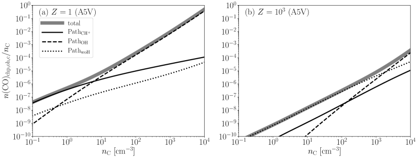
We focus on the high density limit where PathOH is dominant. The path contributes to the CO formation more than . Using the fact that the main destruction processes of OH and CO are photo-dissociation, we obtain the CO fraction as follows: The OH abundance is determined by the balance between the radiative association (the rate coefficient ) and the OH photo-dissociation (the rate coefficient ). Eventually, OH is combined with C to form CO with a rate coefficient of . Considering the CO photo-dissociation (the rate coefficient ), the analytical form of the CO fraction is given by
| (A2) | |||||
where
| (A3) |
, is the oxygen abundance of the gas phase and (Table 1), and we use the fact that and . Equation (A2) shows that the CO fraction depends on , which is quite similar to . The difference between and comes from the temperature dependence shown in Equation (A2).
Equation (A2) shows that is expected to be characterized by at least for high densities where . In order to check this, we fit with a function of , where and are the fitting parameters. As shown in Figure 13, we found that is insensitive to both and for if with and is taken as the horizontal axis. The difference between and with and comes from the negative temperature dependence of (Equation (A2)). The gas temperatures increase when either or increaes. Even for low densities where PathOH is no longer dominant CO formation path, is characterized by reasonably well. A fitting function of the CO fraction is given by
| (A4) |
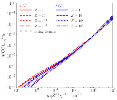
References
- Ádámkovics et al. (2011) Ádámkovics, M., Glassgold, A. E., & Meijerink, R. 2011, ApJ, 736, 143
- Agúndez et al. (2010) Agúndez, M., Goicoechea, J. R., Cernicharo, J., Faure, A., & Roueff, E. 2010, ApJ, 713, 662
- Ahrens & O’Keefe (1972) Ahrens, T. J., & O’Keefe, J. D. 1972, Moon, 4, 214
- Bakes & Tielens (1994) Bakes, E. L. O., & Tielens, A. G. G. M. 1994, ApJ, 427, 822
- Bergin et al. (2016) Bergin, E. A., Du, F., Cleeves, L. I., et al. 2016, ApJ, 831, 101
- Bertoldi & Draine (1996) Bertoldi, F., & Draine, B. T. 1996, ApJ, 458, 222
- Bron et al. (2014) Bron, E., Le Bourlot, J., & Le Petit, F. 2014, A&A, 569, A100
- Burns et al. (1979) Burns, J. A., Lamy, P. L., & Soter, S. 1979, Icarus, 40, 1
- Cataldi et al. (2014) Cataldi, G., Brandeker, A., Olofsson, G., et al. 2014, A&A, 563, A66
- Cataldi et al. (2018) Cataldi, G., Brandeker, A., Wu, Y., et al. 2018, ApJ, 861, 72
- Chen et al. (2006) Chen, C. H., Sargent, B. A., Bohac, C., et al. 2006, ApJS, 166, 351
- Compiègne et al. (2011) Compiègne, M., Verstraete, L., Jones, A., et al. 2011, A&A, 525, A103
- Cuppen et al. (2006) Cuppen, H. M., Morata, O., & Herbst, E. 2006, MNRAS, 367, 1757
- Dent et al. (2014) Dent, W. R. F., Wyatt, M. C., Roberge, A., et al. 2014, Science, 343, 1490
- Dohnanyi (1969) Dohnanyi, J. S. 1969, J. Geophys. Res., 74, 2531
- Draine (1978) Draine, B. T. 1978, ApJS, 36, 595
- Draine & Bertoldi (1996) Draine, B. T., & Bertoldi, F. 1996, ApJ, 468, 269
- Draine & Li (2001) Draine, B. T., & Li, A. 2001, ApJ, 551, 807
- Federman et al. (1979) Federman, S. R., Glassgold, A. E., & Kwan, J. 1979, ApJ, 227, 466
- Fernández et al. (2006) Fernández, R., Brandeker, A., & Wu, Y. 2006, ApJ, 643, 509
- Freudling et al. (1995) Freudling, W., Lagrange, A.-M., Vidal-Madjar, A., Ferlet, R., & Forveille, T. 1995, A&A, 301, 231
- Genda et al. (2015) Genda, H., Kobayashi, H., & Kokubo, E. 2015, ApJ, 810, 136
- Goicoechea & Le Bourlot (2007) Goicoechea, J. R., & Le Bourlot, J. 2007, A&A, 467, 1
- Goicoechea & Roncero (2022) Goicoechea, J. R., & Roncero, O. 2022, A&A, 664, A190
- Goicoechea et al. (2016) Goicoechea, J. R., Pety, J., Cuadrado, S., et al. 2016, Nature, 537, 207
- Gorti et al. (2009) Gorti, U., Dullemond, C. P., & Hollenbach, D. 2009, ApJ, 705, 1237
- Gorti & Hollenbach (2004) Gorti, U., & Hollenbach, D. 2004, ApJ, 613, 424
- Gorti & Hollenbach (2009) —. 2009, ApJ, 690, 1539
- Grigorieva et al. (2007) Grigorieva, A., Thébault, P., Artymowicz, P., & Brandeker, A. 2007, A&A, 475, 755
- Habart et al. (2011) Habart, E., Abergel, A., Boulanger, F., et al. 2011, A&A, 527, A122
- Habing (1968) Habing, H. J. 1968, Bull. Astron. Inst. Netherlands, 19, 421
- Haisch et al. (2001) Haisch, Jr., K. E., Lada, E. A., & Lada, C. J. 2001, ApJ, 553, L153
- Heap et al. (2000) Heap, S. R., Lindler, D. J., Lanz, T. M., et al. 2000, ApJ, 539, 435
- Heays et al. (2017) Heays, A. N., Bosman, A. D., & van Dishoeck, E. F. 2017, A&A, 602, A105
- Herráez-Aguilar et al. (2014) Herráez-Aguilar, D., Jambrina, P. G., Menéndez, M., et al. 2014, Physical Chemistry Chemical Physics (Incorporating Faraday Transactions), 16, 24800
- Hierl et al. (1997) Hierl, P. M., Morris, R. A., & Viggiano, A. A. 1997, J. Chem. Phys., 106, 10145
- Higuchi et al. (2020) Higuchi, A. E., Kóspál, Á., Moór, A., Nomura, H., & Yamamoto, S. 2020, ApJ, 905, 122
- Higuchi et al. (2017) Higuchi, A. E., Sato, A., Tsukagoshi, T., et al. 2017, ApJ, 839, L14
- Higuchi et al. (2019) Higuchi, A. E., Saigo, K., Kobayashi, H., et al. 2019, submitted in ApJ
- Hollenbach et al. (1994) Hollenbach, D., Johnstone, D., Lizano, S., & Shu, F. 1994, ApJ, 428, 654
- Howarth (2011) Howarth, I. D. 2011, MNRAS, 413, 1515
- Hughes et al. (2018) Hughes, A. M., Duchêne, G., & Matthews, B. C. 2018, ARA&A, 56, 541
- Hughes et al. (2008) Hughes, A. M., Wilner, D. J., Kamp, I., & Hogerheijde, M. R. 2008, ApJ, 681, 626
- Hughes et al. (2017) Hughes, A. M., Lieman-Sifry, J., Flaherty, K. M., et al. 2017, ApJ, 839, 86
- Hunter (2007) Hunter, J. D. 2007, Computing in Science and Engineering, 9, 90
- Ivanovskaya et al. (2010) Ivanovskaya, V. V., Zobelli, A., Teillet-Billy, D., et al. 2010, Phys. Rev. B, 82, 245407
- Iwasaki et al. (2001) Iwasaki, K., Tanaka, H., Nakazawa, K., & Hiroyuki, E. 2001, PASJ, 53, 321
- Joblin et al. (2018) Joblin, C., Bron, E., Pinto, C., et al. 2018, A&A, 615, A129
- Jura (1974) Jura, M. 1974, ApJ, 191, 375
- Jura et al. (1998) Jura, M., Malkan, M., White, R., et al. 1998, ApJ, 505, 897
- Jura et al. (1993) Jura, M., Zuckerman, B., Becklin, E. E., & Smith, R. C. 1993, ApJ, 418, L37
- Kama et al. (2016) Kama, M., Bruderer, S., van Dishoeck, E. F., et al. 2016, A&A, 592, A83
- Kamp & Bertoldi (2000) Kamp, I., & Bertoldi, F. 2000, A&A, 353, 276
- Kamp et al. (2003) Kamp, I., van Zadelhoff, G.-J., van Dishoeck, E. F., & Stark, R. 2003, A&A, 397, 1129
- Kobayashi & Löhne (2014) Kobayashi, H., & Löhne, T. 2014, MNRAS, 442, 3266
- Kobayashi & Tanaka (2010) Kobayashi, H., & Tanaka, H. 2010, Icarus, 206, 735
- Kobayashi et al. (2008) Kobayashi, H., Watanabe, S., Kimura, H., & Yamamoto, T. 2008, Icarus, 195, 871
- Kobayashi et al. (2009) —. 2009, Icarus, 201, 395
- Kóspál et al. (2013) Kóspál, Á., Moór, A., Juhász, A., et al. 2013, ApJ, 776, 77
- Kral et al. (2019) Kral, Q., Marino, S., Wyatt, M. C., Kama, M., & Matrà, L. 2019, MNRAS, 489, 3670
- Kral et al. (2017) Kral, Q., Matrà, L., Wyatt, M. C., & Kennedy, G. M. 2017, MNRAS, 469, 521
- Kral et al. (2016) Kral, Q., Wyatt, M., Carswell, R. F., et al. 2016, MNRAS, 461, 845
- Kraus et al. (2011) Kraus, R. G., Senft, L. E., & Stewart, S. T. 2011, Icarus, 214, 724
- Kurosawa et al. (2010) Kurosawa, K., Sugita, S., Kadono, T., et al. 2010, Geophys. Res. Lett., 37, L23203
- Kurucz (1992) Kurucz, R. L. 1992, Rev. Mexicana Astron. Astrofis., 23, 181
- Laor & Draine (1993) Laor, A., & Draine, B. T. 1993, ApJ, 402, 441
- Lavendy et al. (1993) Lavendy, H., Robbe, J. M., & Flament, J. P. 1993, Chemical Physics Letters, 205, 456
- Le Bourlot et al. (2012) Le Bourlot, J., Le Petit, F., Pinto, C., Roueff, E., & Roy, F. 2012, A&A, 541, A76
- Le Petit et al. (2009) Le Petit, F., Barzel, B., Biham, O., Roueff, E., & Le Bourlot, J. 2009, A&A, 505, 1153
- Le Petit et al. (2006) Le Petit, F., Nehmé, C., Le Bourlot, J., & Roueff, E. 2006, ApJS, 164, 506
- Lecavelier des Etangs et al. (2001) Lecavelier des Etangs, A., Vidal-Madjar, A., Roberge, A., et al. 2001, Nature, 412, 706
- Lodders (2008) Lodders, K. 2008, ApJ, 674, 607
- Mathis et al. (1983) Mathis, J. S., Mezger, P. G., & Panagia, N. 1983, A&A, 128, 212
- Mathis et al. (1977) Mathis, J. S., Rumpl, W., & Nordsieck, K. H. 1977, ApJ, 217, 425
- Matrà et al. (2015) Matrà, L., Panić, O., Wyatt, M. C., & Dent, W. R. F. 2015, MNRAS, 447, 3936
- Matrà et al. (2018) Matrà, L., Wilner, D. J., Öberg, K. I., et al. 2018, ApJ, 853, 147
- Matrà et al. (2017) Matrà, L., Dent, W. R. F., Wyatt, M. C., et al. 2017, MNRAS, 464, 1415
- Mennella (2006) Mennella, V. 2006, ApJ, 647, L49
- Meyer et al. (1997) Meyer, D. M., Cardelli, J. A., & Sofia, U. J. 1997, ApJ, 490, L103
- Meyer et al. (1998) Meyer, D. M., Jura, M., & Cardelli, J. A. 1998, ApJ, 493, 222
- Mizuno et al. (1978) Mizuno, H., Nakazawa, K., & Hayashi, C. 1978, Progress of Theoretical Physics, 60, 699
- Montesinos et al. (2009) Montesinos, B., Eiroa, C., Mora, A., & Merín, B. 2009, A&A, 495, 901
- Moór et al. (2019) Moór, A., Kral, Q., Ábrahám, P., et al. 2019, ApJ, 884, 108
- Morton (1975) Morton, D. C. 1975, ApJ, 197, 85
- Nakatani et al. (2018) Nakatani, R., Hosokawa, T., Yoshida, N., Nomura, H., & Kuiper, R. 2018, ApJ, 865, 75
- Nakatani et al. (2021) Nakatani, R., Kobayashi, H., Kuiper, R., Nomura, H., & Aikawa, Y. 2021, ApJ, 915, 90
- Navarro-Ruiz et al. (2015) Navarro-Ruiz, J., Martínez-González, J. Á., Sodupe, M., Ugliengo, P., & Rimola, A. 2015, MNRAS, 453, 914
- Navarro-Ruiz et al. (2014) Navarro-Ruiz, J., Sodupe, M., Ugliengo, P., & Rimola, A. 2014, Physical Chemistry Chemical Physics (Incorporating Faraday Transactions), 16, 17447
- Okeefe & Ahrens (1982) Okeefe, J. D., & Ahrens, T. J. 1982, J. Geophys. Res., 87, 6668
- Ootsubo et al. (2012) Ootsubo, T., Kawakita, H., Hamada, S., et al. 2012, ApJ, 752, 15
- Owen et al. (2012) Owen, J. E., Clarke, C. J., & Ercolano, B. 2012, MNRAS, 422, 1880
- Roberge et al. (2000) Roberge, A., Feldman, P. D., Lagrange, A. M., et al. 2000, ApJ, 538, 904
- Roberge et al. (2006) Roberge, A., Feldman, P. D., Weinberger, A. J., Deleuil, M., & Bouret, J.-C. 2006, Nature, 441, 724
- Roberge et al. (2013) Roberge, A., Kamp, I., Montesinos, B., et al. 2013, ApJ, 771, 69
- Savage & Sembach (1996) Savage, B. D., & Sembach, K. R. 1996, ARA&A, 34, 279
- Sha et al. (2002) Sha, X., Jackson, B., & Lemoine, D. 2002, J. Chem. Phys., 116, 7158
- Sternberg et al. (2021) Sternberg, A., Gurman, A., & Bialy, S. 2021, ApJ, 920, 83
- Sultanov & Balakrishnan (2005) Sultanov, R. A., & Balakrishnan, N. 2005, ApJ, 629, 305
- Suzuki & Inutsuka (2009) Suzuki, T. K., & Inutsuka, S.-i. 2009, ApJ, 691, L49
- Suzuki & Inutsuka (2014) —. 2014, ApJ, 784, 121
- Tanaka et al. (1996) Tanaka, H., Inaba, S., & Nakazawa, K. 1996, Icarus, 123, 450
- Tanigawa & Ikoma (2007) Tanigawa, T., & Ikoma, M. 2007, ApJ, 667, 557
- Tieftrunk et al. (1994) Tieftrunk, A., Pineau des Forets, G., Schilke, P., & Walmsley, C. M. 1994, A&A, 289, 579
- van der Walt et al. (2011) van der Walt, S., Colbert, S. C., & Varoquaux, G. 2011, Computing in Science and Engineering, 13, 22
- van Dishoeck & Black (1988) van Dishoeck, E. F., & Black, J. H. 1988, ApJ, 334, 771
- van Dishoeck & Dalgarno (1983) van Dishoeck, E. F., & Dalgarno, A. 1983, J. Chem. Phys., 79, 873
- van Dishoeck & Dalgarno (1984) —. 1984, ApJ, 277, 576
- van Dishoeck et al. (2006) van Dishoeck, E. F., Jonkheid, B., & van Hemert, M. C. 2006, Faraday Discussions, 133, 231
- Veselinova et al. (2021) Veselinova, A., Agúndez, M., Goicoechea, J. R., et al. 2021, A&A, 648, A76
- Visser et al. (2009) Visser, R., van Dishoeck, E. F., & Black, J. H. 2009, A&A, 503, 323
- Weaver et al. (2011) Weaver, H. A., Feldman, P. D., A’Hearn, M. F., Dello Russo, N., & Stern, S. A. 2011, ApJ, 734, L5
- Wishart (1979) Wishart, A. W. 1979, MNRAS, 187, 59P
- Zanchet et al. (2013a) Zanchet, A., Agúndez, M., Herrero, V. J., Aguado, A., & Roncero, O. 2013a, AJ, 146, 125
- Zanchet et al. (2013b) Zanchet, A., Godard, B., Bulut, N., et al. 2013b, ApJ, 766, 80
- Zecho et al. (2002) Zecho, T., Guttler, A., Sha, X., Jackson, B., & Kuppers, J. 2002, J. Chem. Phys., 117, 8486