A Constrained Mean Curvature Flow On Capillary Hypersurface Supported on totally geodesic plane

Mean curvature flow has a rich history, dating back to significant works such as Huisken [13]. Huisken showed that a convex and closed hypersurface will flow to a sphere under the properly rescaled mean curvature flow. A constrained curvature flow is a flow which preserves some geometric quantities. In $\mathbb{R}^{2}$, Gage  [5] used a constrained curve shortening flow to prove an isoperimetric inequality. In higher dimensions, a constrained mean curvature flow was applied to prove the isoperimetric inequality by Huisken [14]. This constrained flow preserves the enclosed volume while decreasing the area of the hypersurface.

An alternative approach to create a flow that preserves the enclosed volume is by employing the Minkowski formula on the hypersurface. This has been explored in [6], which investigated such flows in space forms. Furthermore, this approach has been extended to warped product spaces in [7], where they considered the flow $x:(\mathbb{R}\times N,g)\rightarrow(\bar{M},\bar{g}=dr^{2}+\phi^{2}(r)g_{N})$ satisfying

$$\frac{\partial x}{\partial t}=(n\phi^{\prime}-uH)\nu.$$

Under appropriate assumptions on the metric $\bar{g}$, the flow is expected to converge to a level set of $\phi$. See for example [1], [2], [3], [9] and [10] for various types of fully nonlinear curvature flow and anisotropic curvature flow in different ambient spaces.

In recent years, there has been considerable interest in geometric flows of capillary hypersurfaces, for instance, inverse mean curvature flow with free boundary in the Euclidean unit ball [15].

Diving into the main topic of this paper, constrained curvature flow on capillary hypersurfaces has yielded significant results. These include: constrained inverse mean curvature type [19], [23] and mean curvature type flow [12], [20] for capillary hypersurfaces in the Euclidean unit ball; curvature flows [11], [16] and [21] in capillary hypersurfaces in Euclidean half space;  mean curvature type flow [17] in geodesic ball in space forms.

In this paper, we consider a new constrained mean curvature type flow for capillary hypersurfaces, which are supported on totally geodesic hyperplanes in hyperbolic space $\mathbb{H}^{n+1}$. We use the well-known Poincar$\acute{\mathrm{e}}$ half space model $(\mathbb{H}^{n+1},\langle\cdot,\cdot\rangle)=\left(\mathbb{R}^{n+1}_{+},\frac{1}{x^{2}_{n+1}}\langle\cdot,\cdot\rangle_{\delta}\right)$, where $x_{n+1}$ is the $(n+1)$-th coordinate, $\langle\cdot,\cdot\rangle_{\delta}$ is the Euclidean metric and $\mathbb{R}^{n+1}_{+}:=\{x\in\mathbb{R}^{n+1}:x_{n+1}>0\}$. Let $P:=\{x\in\mathbb{H}^{n+1}:x_{1}=0\}$ be a totally geodesic hyperplane. Denote by $x$ the position vector in $\mathbb{R}^{n+1}_{+}$and $\{E_{i}\}_{i=1}^{n+1}$ the coordinate basis of $(\mathbb{R}^{n+1},\langle\cdot,\cdot\rangle_{\delta})$.

Throughout the paper, we consider $x_{0}:M\rightarrow\mathbb{H}^{n+1}$ as an immersion of hypersurface in $\mathbb{H}^{n+1}$. If $\Sigma=x(M)$ satisfies that

1. i.

   $\operatorname{int}\Sigma=x(\operatorname{int}M)\subset P_{+}:=\{x\in\mathbb{H}^{n+1}:x_{1}>0\}$,

2. ii.

   $\partial\Sigma=x(\partial M)\subset\{x\in\mathbb{H}^{n+1}:x_{1}=0\}=P$,

3. iii.

   $\Sigma$ and $P$ contacts at a constant angle $\theta$ on $\partial\Sigma=\Sigma\cap P$,

we call $\Sigma$ a $\theta$-capillary hypersurface supported on $P$, and $P$ the supporting hypersurface.

On a $\theta$-capillary hypersurface supported on totally geodesic hyperplane $P$, we introduce a novel condition called star-shapedness with respect to $cE_{n+1}$.

We consider a flow, defined as a family of embeddings $x:M\times[0,T)\rightarrow\mathbb{H}^{n+1}$ with $x(\partial\Sigma,\cdot)\subset P$, such that

(1)

$$\begin{array}[]{rclccl}(\partial_{t}x)^{\bot}&=&q_{c}\nu,&&&\operatorname{in}M\times[0,T);\\ \langle\nu,\bar{N}\circ x\rangle&=&-\cos\theta,&&&\operatorname{on}\partial M\times[0,T);\\ x(\cdot,0)&=&x_{0}(\cdot),&&&\operatorname{on}M,\end{array}$$

where the normal velocity $q_{c}$ is given by

$$q_{c}=\frac{nc}{x_{n+1}}-nc\cos\theta\langle E_{1},\nu\rangle-H\langle x-cE_{n+1},\nu\rangle.$$

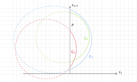
We denote by $\kappa$ the principal curvature of an umbilical hypersurface $\mathcal{C}$. Umbilical hypersurfaces in hyperbolic space can be classified into three types depending on $\kappa$ as depicted in the figure. In the case of $\kappa=0$, it is a totally geodesic hyperplane; in the case of $\kappa>1$, it is a geodesic sphere, and for $0<\kappa<1$, it is an equidistant hypersurface, and if $\kappa=1$, it is a horosphere. In the Poincaré half space model, $\mathcal{C}$ can be represented as a plane or sphere with respect to the Euclidean metric. It is easy to see that compact umbilical $\theta$-capillary hypersurface, can be part of a geodesic sphere, a horosphere and an equidistant hypersurface.

To state our main theorem, we need the following definition.

For a $\theta$-umbilical cap, we define a constant $K_{0}(c,R,\theta)$ by

$$K_{0}(c,R,\theta)=\left\{\begin{array}[]{llll}c-R\sin\theta&&&\theta\leq\pi/2\\ c-R&&&\theta>\pi/2\end{array}\right..$$

Note that $K_{0}(c,R,\theta)>0$ if and only if the $\mathcal{C}_{c,R,\theta}(a)$ is compact. Combining with Remark 2, we know that its principal curvature $\kappa=\frac{c}{R}>\sin\theta$.

Now we are ready to state our main theorem.

The following remark is crucial, which shows that some specific umbilical caps are static along the flow (1).

The paper is organized as follows:

In Section 2, we introduce basic notations and definitions of hypersurfaces. In Section 3, we prove a new Minkowski formula on capillary hypersurface supported on a totally geodesic hyperplane, comparing to the one in [4]. In Sections 4, 5 and 6, we follow the method in [20] and [16] to study the scalar equation of the flow (1), in particular, we prove the $C^{0}$ and $C^{1}$ estimates. In Section 7, we prove the uniform convergence of the flow.

Throughout this paper, we assume that $x:M\rightarrow P_{+}\subset\mathbb{H}^{n+1}$ is an embedding of capillary hypersurface along $P$. We denote the second fundamental form of the embedding by $h_{ij}$. Since $\nu$ is the outer normal field on $\Sigma$, $h_{ij}=\langle\nabla_{e_{i}}\nu,e_{j}\rangle$. Let $\kappa=(\kappa_{1},\cdots,\kappa_{n})$ be the eigenvalues of $(h_{ij})$, i.e., the principal curvatures of $\Sigma$. The $k$-th mean curvature $S_{k}$ is defined by

$$S_{r}=\frac{1}{r!}\sum_{1\leq i_{1}<\cdots<i_{r}\leq n}\kappa_{1}\kappa_{2}\cdots\kappa_{i_{r}},$$

and the normalized mean curvature is defined by $H_{r}=\binom{n}{r}^{-1}S_{r}$.

The following so-called Newton transformation defined on the tangent bundle is essential to our formula:

$$T_{0}=\operatorname{id},$$

$$T_{k}=S_{k}I-T_{k-1}\circ h.$$

The following properties are well-known,

$$\operatorname{tr}(T_{r})=(n-r)S_{r}=(n-r)\binom{n}{r}H_{r},$$

$$\operatorname{tr}(T_{r}\circ h)=(r+1)S_{r+1}=(n-k)\binom{n}{r}H_{r+1}.$$

Let $\bar{N}$ denote the outer normal field of $P$ ($P_{+}$ is the interior side), $\nu$ denote the outer normal field of the immersed hypersurface $\Sigma$, $\bar{\nu}$ denote the outer normal field of $\partial\Sigma\subset P$ and $\eta$ denote the outer conormal field along $\partial\Sigma\subset\Sigma$. Without loss of generality, assuming $\theta$ as the angle between $-\nu$ and $\bar{N}$, we have the following relation

(4)

$$\left\{\begin{array}[]{l}\mu=\sin\theta\overline{N}+\cos\theta\overline{\nu}\\ \nu=-\cos\theta\overline{N}+\sin\theta\overline{\nu}\end{array}\right..$$

Then the following lemma is widely recognized, and we refer to [22] for its proof.

This property of capillary hypersurfaces is essential in the proof of the Minkowski type formula in the next section.

In this section, we introduce a new Minkowski type formula, which is based on the the following properties (see [8]).

These can be directly calculated by the relation between Levi-Civita connections of the metrics conformal to each other, we refer the proof to [8]. From (6), (8), and (9), we can easily see that $x$, $E_{1}$, and $E_{n+1}$ are conformal Killing vector fields, that is,

(11)

$$(\mathcal{L}_{x}\bar{g})(X,Y)=\frac{1}{2}(\langle\overline{\nabla}_{Y}x,X\rangle+\langle\overline{\nabla}_{X}x,Y\rangle)=0,$$

(12)

$$(\mathcal{L}_{E_{1}}\bar{g})(X,Y)=\frac{1}{2}(\langle\overline{\nabla}_{Y}E_{1},X\rangle+\langle\overline{\nabla}_{X}E_{1},Y\rangle)=0,$$

and

(13)

$$\begin{array}[]{ccl}\mathcal{L}_{-E_{n+1}}\langle X,Y\rangle&=&\frac{1}{2}(\langle\overline{\nabla}_{Y}(-E_{n+1}),X\rangle+\langle\overline{\nabla}_{X}(-E_{n+1}),Y\rangle)\\ &=&\frac{1}{x_{n+1}}\langle X,Y\rangle,\end{array}$$

for any $X,Y\in T\mathbb{H}^{n+1}$, where $\bar{g}$ denotes the metric $\langle\cdot,\cdot\rangle$.

Restricting the equation (13) to $T\Sigma$, we have

(14)

$$\langle\nabla^{\Sigma}_{e_{i}}E_{1},e_{j}\rangle=-\langle e_{i},\overline{E}_{n+1}\rangle\langle E_{1},e_{j}\rangle+\langle e_{i},E_{1}\rangle\langle\overline{E}_{n+1},e_{j}\rangle-h_{ij}\langle E_{1}{,}\nu\rangle,$$

(15)

$$\langle\nabla^{\Sigma}_{e_{i}}x,e_{j}\rangle=-\langle e_{i},\overline{E}_{n+1}\rangle\langle x,e_{j}\rangle+\langle e_{i},x\rangle\langle\overline{E}_{n+1},e_{j}\rangle-h_{ij}\langle x{,}\nu\rangle,$$

and

(16)

$$\langle\nabla^{\Sigma}_{e_{i}}(-E_{n+1}),e_{j}\rangle=\frac{1}{x_{n+1}}\langle e_{i},e_{j}\rangle-h_{ij}\langle-E_{n+1}{,}\nu\rangle.$$

Let $x:\Sigma\rightarrow(\mathbb{H}^{n+1},\langle\cdot,\cdot\rangle)=\left(\mathbb{R}^{n+1}_{+},\frac{1}{x^{2}_{n+1}}\langle\cdot,\cdot\rangle_{\delta}\right)$ be an immersion of $\theta$-capillary hypersurface supported on the hyperplane $P$. By using the facts above, we can prove the following Minkowski type formula on $\Sigma$.

Let $k=1$, the Minkowski formula (17) becomes

(18)

$$\int_{\Sigma}\left[nc\left(\frac{1}{x_{n+1}}-\cos\theta\langle E_{1},\nu\rangle\right)-H\langle x-cE_{n+1},\nu\rangle\right]dA=0,$$

which holds for any capillary hypersurfaces $\Sigma$ supported on totally geodesic hyperplane $P$. Here $H=nH_{1}$ is the mean curvature of $\Sigma$.

Let $\hat{\Sigma}$ denote the domain enclosed by $\Sigma$ and $P$, and $|\widehat{\partial\Sigma}|$ be the domain enclosed by $\partial\Sigma$ on $P$. The energy functional defined by

$$\mathcal{Q}(\Sigma)=|\Sigma|-\cos\theta|\widehat{\partial\Sigma}|$$

is well-known since the critical hypersurface of this functional under any volume preserving variation is a $\theta$-capillary hypersurface with constant mean curvature, see [18] and [22]. Under a flow $\Sigma_{t}=x_{t}(M)$ with with the given normal velocity $f$ and capillary boundary condition as in (1), the following variation formula is well-known:

$$\frac{d}{dt}|\hat{\Sigma}_{t}|=\int_{\Sigma_{t}}fdA_{t}$$

and

$$\frac{d}{dt}\mathcal{Q}(\Sigma_{t})=\text{$\int_{\Sigma_{t}}HfdA_{t}.$}$$

From the Minkowski formula $\eqref{Mink}$, it is evident that the flow described in (1) is a volume preserving flow.

In this section, we express the flow (1) by a scalar equation of the radius function.

Let $x$ be the position vector defined on $M$ which is represented by

$$x=cE_{n+1}+\rho(z)z,z\in\Omega\subset\bar{\mathbb{S}}^{n}_{+},$$

where $\rho$ defined on $\mathbb{S}^{n}_{+}$ is the distance between $x$ and $cE_{n+1}$ in the Euclidean metric. Since $\Sigma$ is smooth, star-shaped, the function $\rho$ is well-defined and smooth on $\Omega$. Let $u=\log\rho$, then $u\in C^{2}(\Omega)\cap C^{0}(\bar{\Omega})$. Define $v=\sqrt{1+|\nabla u|^{2}}$, where $\nabla u$ is the gradient of $u$ with respect to the ordinary metric on $\mathbb{S}^{n}_{+}$. From the basic facts for radial function, it is well-known that

$$\tilde{\nu}:=x^{-1}_{n+1}\nu=\frac{\zeta-\rho^{-1}\nabla u}{v},$$

where $\zeta=\partial_{\rho}$.

Throughout the paper, we let the indices $i,j,k$ range from 1 to $n$ and we will apply the Einstein convention.

We use polar coordinates $(\rho,\beta,\gamma,\xi)\in[0,+\infty)\times\left[0,\frac{\pi}{2}\right]\times[0,2\pi]\times\mathbb{S}^{n-2}$, where $\xi$ is the spherical coordinate on $\mathbb{S}^{n-2}$, and the star-shaped hypersurface $\Sigma:=x(M)$ can be written as

(20)

$$x-cE_{n+1}=\rho(z)z=\rho(\beta,\gamma,\xi)z,\hskip 18.00005pt\operatorname{where}z:=(\beta,\gamma,\xi)\in\bar{\mathbb{S}}_{+}^{n},$$

where $x_{1}=\rho\cos\beta$ and $x_{n+1}=\rho\sin\beta\cos\gamma+c=e^{-w}$. Then the Euclidean metric $ds^{2}=\langle\cdot,\cdot\rangle_{\delta}$ can be written as

$$ds^{2}=d\rho^{2}+\rho^{2}\sigma_{\mathbb{S}^{n}_{+}}=d\rho^{2}+\rho^{2}d\beta^{2}+\rho^{2}\sin^{2}\beta d\gamma^{2}+\rho^{2}\sin^{2}\beta\sin^{2}\gamma\sigma_{\mathbb{S}^{n-2}},$$

and we have

$$\rho^{2}=x_{1}^{2}+\sum_{i=2}^{n}x_{i}^{2}+(x_{n+1}-c)^{2}.$$

Now we can represent $E_{1}$, $E_{n+1}$ by the coordinate (20). Indeed, since

$$\frac{\partial\rho}{\partial x_{1}}=\frac{x_{1}}{\rho}=\cos\beta,$$

and

$$-\sin\beta\frac{\partial\beta}{\partial x_{1}}=\frac{\partial(\cos\beta)}{\partial x_{1}}=\frac{\partial(x_{1}/\rho)}{\partial x_{1}}=\frac{\sin^{2}\beta}{\rho},$$

we can represent $E_{1}$ by the polar coordinate defined above,

(21)

$$E_{1}=\frac{\partial}{\partial x_{1}}=\frac{\partial\rho}{\partial x_{1}}\partial_{\rho}+\frac{\partial\beta}{\partial x_{1}}\partial_{\beta}=\cos\beta\partial_{\rho}-\frac{\sin\beta}{\rho}\partial_{\beta}.$$

Similarly, since

$$\frac{\partial\rho}{\partial x_{n+1}}=\frac{x_{n+1}-c}{\rho}=\sin\beta\cos\gamma,$$

$$-\sin\beta\frac{\partial\beta}{\partial x_{n+1}}=\frac{\partial(\cos\beta)}{\partial x_{n+1}}=\frac{\partial(x_{1}/\rho)}{\partial x_{n+1}}=-\frac{1}{\rho}\sin\beta\cos\beta\cos\gamma$$

and

$$-\sin\gamma\frac{\partial\gamma}{\partial x_{n+1}}=\frac{\partial(\cos\gamma)}{\partial x_{n+1}}=\frac{\partial((x_{n+1}-c)/(\rho\sin\beta))}{\partial x_{n+1}}=\frac{\sin^{2}\gamma}{\rho\sin\beta},$$

we have

(22)

$$E_{n+1}=\frac{\partial}{\partial x_{n+1}}=\sin\beta\cos\gamma\partial_{\rho}+\frac{1}{\rho}\cos\beta\cos\gamma\partial_{\beta}-\frac{\sin\gamma}{\rho\sin\beta}\partial_{\gamma}.$$

Denoting $u_{\beta}=\sigma(\nabla u,\partial_{\beta})$ and $u_{\gamma}=\sigma(\nabla u,\partial_{\gamma})$, from (21) and (22) we have

(23)

$$\langle E_{1},\nu\rangle=e^{2w}\langle\cos\beta\partial_{\rho}-\frac{\sin\beta}{\rho}\partial_{\beta},e^{-w}\frac{\zeta-\rho^{-1}\nabla u}{v}\rangle_{\delta}=e^{w}\frac{\cos\beta-\sin\beta u_{\beta}}{v},$$

and

(24)		$\displaystyle\langle E_{n+1},\tilde{\nu}\rangle_{\delta}=$	$\displaystyle\langle\sin\beta\cos\gamma\partial_{\rho}+\frac{1}{\rho}\cos\beta\cos\gamma\partial_{\beta}-\frac{\sin\gamma}{\rho\sin\beta}\partial_{\gamma},\frac{\zeta-\rho^{-1}\nabla u}{v}\rangle_{\delta}$
		$\displaystyle=$	$\displaystyle\frac{1}{v}(\sin\beta\cos\gamma-\cos\beta\cos\gamma u_{\beta}+\sin\beta\sin\gamma u_{\gamma}).$

By definition, we have

(25)

$$\langle x-cE_{n+1},\nu\rangle=e^{2w}\langle\rho\zeta,e^{-w}\frac{\zeta-\rho^{-1}\nabla u}{v}\rangle=\frac{\rho e^{w}}{v}.$$

Moreover, by the conformality of mean curvature,

(26)		$\displaystyle H=$	$\displaystyle e^{-w}\left[\frac{n}{\rho v}-\frac{1}{\rho v}\left(\sigma^{ij}-\frac{u^{i}u^{j}}{v^{2}}\right)u_{ij}\right]-nD_{\tilde{\nu}}e^{-w}$
		$\displaystyle=$	$\displaystyle e^{-w}\left[\frac{n}{\rho v}-\frac{1}{\rho v}\left(\sigma^{ij}-\frac{u^{i}u^{j}}{v^{2}}\right)u_{ij}\right]-n\langle E_{n+1},\tilde{\nu}\rangle_{\delta}$
		$\displaystyle=$	$\displaystyle-\frac{1}{\rho ve^{w}}\left(\sigma^{ij}-\frac{u^{i}u^{j}}{v^{2}}\right)u_{ij}+\frac{1}{v}(\cos\beta\cos\gamma u_{\beta}-\sin\beta\sin\gamma u_{\gamma})+\frac{nc}{\rho v},$

where $\sigma^{ij}$ corresponds to the inverse of the metric on $\mathbb{S}^{n}_{+}$, $u^{i}=\sigma^{ij}u_{j}$ is the $i$-th component of $\nabla u$ (the gradient of $u$ on $\mathbb{S}^{n}_{+}$) and $u_{ij}$ is the $(i,j)$-th component of the Hessian $\nabla^{2}u$ on $\mathbb{S}^{n}_{+}$. Then by calculation,

	$\displaystyle q_{c}$	$\displaystyle=$	$\displaystyle nc\left(\frac{1}{x_{n+1}}-\cos\theta\langle E_{1},\nu\rangle\right)-H\langle x-cE_{n+1},\nu\rangle$
		$\displaystyle=$	$\displaystyle nce^{w}-nc\cos\theta v^{-1}e^{w}(\cos\theta-\sin\beta u_{\beta})$
			$\displaystyle-\left(-\frac{1}{\rho ve^{w}}\left(\sigma^{ij}-\frac{u^{i}u^{j}}{v^{2}}\right)u_{ij}+\frac{1}{v}(\cos\beta\cos\gamma u_{\beta}-\sin\beta\sin\gamma u_{\gamma})+\frac{nc}{\rho v}\right)\frac{\rho e^{w}}{v}.$

Writing the flow as a function $u$ of $t$, from the flow (1), we see that

$$q_{c}=\langle\partial_{t}x,\nu\rangle=\rho_{t}e^{-w}e^{2w}\langle\zeta,\frac{\zeta-\rho^{-1}\nabla u}{\sqrt{1+|\nabla u|^{2}}}\rangle_{\delta}=\frac{\rho_{t}e^{w}}{\sqrt{1+|\nabla u|^{2}}}=\frac{u_{t}\rho e^{w}}{v}.$$

Therefore, we obtain the evolution equation of $u$ as follows,

(27)		$\displaystyle u_{t}=$	$\displaystyle\frac{v}{\rho e^{w}}q_{c}$
		$\displaystyle=$	$\displaystyle\frac{ncv}{\rho}-\frac{nc\cos\theta}{\rho}(\cos\beta-\sin\beta u_{\beta})+\frac{1}{\rho e^{w}v}\left(\sigma^{ij}-\frac{u^{i}u^{j}}{v^{2}}\right)u_{ij}$
			$\displaystyle+\frac{n}{v}(-\cos\beta\cos\gamma u_{\beta}+\sin\beta\sin\gamma u_{\gamma})-\frac{nc}{\rho v}$
		$\displaystyle=$	$\displaystyle\frac{nc}{\rho}\frac{|\nabla u|^{2}}{v}-\frac{nc\cos\theta}{\rho}(\cos\beta-\sin\beta u_{\beta})$
			$\displaystyle+\frac{1}{\rho e^{w}v}\left(\sigma^{ij}-\frac{u^{i}u^{j}}{v^{2}}\right)u_{ij}+\frac{n}{v}(-\cos\beta\cos\gamma u_{\beta}+\sin\beta\sin\gamma u_{\gamma})$
		$\displaystyle=:$	$\displaystyle Q_{c}(\nabla^{2}u,\nabla u,\rho,\beta,\gamma).$

As for the boundary condition in (1),

	$\displaystyle-\cos\theta$	$\displaystyle=\langle\nu,\bar{N}\rangle$
		$\displaystyle=e^{2w}\langle e^{-w}\tilde{\nu},-e^{-w}E_{1}\rangle_{\delta}$
		$\displaystyle=\langle\frac{\zeta-\rho^{-1}\nabla u}{v},\frac{1}{\rho}\partial_{\beta}\rangle_{\delta}$
		$\displaystyle=-\frac{1}{v}u_{\beta}.$

Therefore we have

(28)

$$u_{\beta}=\rho v\cos\theta=\sqrt{1+|\nabla u|^{2}}\cos\theta.$$

Combining (27) and (28), we know that the flow (1) can be written as the parabolic equation of the scalar function $u$ as follows,

(29)

$$\left\{\begin{array}[]{lllll}u_{t}=Q_{c}(\nabla^{2}u,\nabla u,\rho,\beta,\gamma),&&&\operatorname{in}&\mathbb{S}^{n}_{+}\times[0,T);\\ u_{\beta}=\sqrt{1+|\nabla u|^{2}}\cos\theta,&&&\operatorname{on}&\partial\mathbb{S}^{n}_{+}\times[0,T);\\ u(\cdot,0)=u_{0}(.),&&&\operatorname{on}&\mathbb{S}^{n}_{+},\end{array}\right.$$

where $u_{0}=\log\rho_{0}$ and $\rho_{0}=|x_{0}-cE_{n+1}|_{\delta}$ is the radial function with respect to $cE_{n+1}$ of the initial hypersurface $\Sigma_{0}=x_{0}(M)$.

References

- [1] Ben Andrews “Volume-preserving anisotropic mean curvature flow” In Indiana University mathematics journal JSTOR, 2001, pp. 783–827
- [2] Ben Andrews and Yong Wei “Quermassintegral preserving curvature flow in hyperbolic space” In Geometric and Functional Analysis 28.5 Springer, 2018, pp. 1183–1208
- [3] Ben Andrews and Yong Wei “Volume preserving flow by powers of the th mean curvature” In Journal of Differential Geometry 117.2 Lehigh University, 2021, pp. 193–222
- [4] Yimin Chen and Juncheol Pyo “Some rigidity results on compact hypersurfaces with capillary boundary in Hyperbolic space” In arXiv preprint arXiv:2206.09062, 2022
- [5] Michael Gage “On an area-preserving evolution equation for plane curves” In Nonlinear problems in geometry 51 American Mathematical Society, 1986, pp. 51–62
- [6] Pengfei Guan and Junfang Li “A mean curvature type flow in space forms” In International Mathematics Research Notices 2015.13 Oxford University Press, 2015, pp. 4716–4740
- [7] Pengfei Guan, Junfang Li and Mu-Tao Wang “A volume preserving flow and the isoperimetric problem in warped product spaces” In Transactions of the American Mathematical Society 372.4, 2019, pp. 2777–2798
- [8] Jinyu Guo, Guofang Wang and Chao Xia “Stable capillary hypersurfaces supported on a horosphere in the hyperbolic space” In Adv. Math. 409, Part A Elsevier, 2022, pp. 108641
- [9] Yingxiang Hu and Haizhong Li “Geometric inequalities for static convex domains in hyperbolic space” In Transactions of the American Mathematical Society 375.08, 2022, pp. 5587–5615
- [10] Yingxiang Hu, Haizhong Li and Yong Wei “Locally constrained curvature flows and geometric inequalities in hyperbolic space” In Mathematische Annalen 382.3 Springer, 2022, pp. 1425–1474
- [11] Yingxiang Hu, Yong Wei, Bo Yang and Tailong Zhou “A complete family of Alexandrov-Fenchel inequalities for convex capillary hypersurfaces in the half-space” In arXiv preprint arXiv:2209.12479, 2022
- [12] Yingxiang Hu, Yong Wei, Bo Yang and Tailong Zhou “On the mean curvature type flow for convex capillary hypersurfaces in the ball” In Calculus of Variations and Partial Differential Equations 62.7 Springer, 2023, pp. 209
- [13] Gerhard Huisken “Flow by mean curvature of convex surfaces into spheres” In Journal of Differential Geometry 20.1 Lehigh University, 1984, pp. 237–266
- [14] Gerhard Huisken “The volume preserving mean curvature flow.” In Journal für die reine und angewandte Mathematik 1987.382, 1987, pp. 35–48 DOI: doi:10.1515/crll.1987.382.35
- [15] Ben Lambert and Julian Scheuer “The inverse mean curvature flow perpendicular to the sphere” In Mathematische Annalen 364 Springer, 2016, pp. 1069–1093
- [16] Xinqun Mei, Guofang Wang and Liangjun Weng “A Constrained Mean Curvature Flow and Alexandrov–Fenchel Inequalities” In International Mathematics Research Notices 2024.1 Oxford University Press, 2024, pp. 152–174
- [17] Xinqun Mei and Liangjun Weng “A constrained mean curvature type flow for capillary boundary hypersurfaces in space forms” In The Journal of Geometric Analysis 33.6 Springer, 2023, pp. 195
- [18] Antonio Ros and Rabah Souam “On stability of capillary surfaces in a ball” In pacific journal of mathematics 178.2 Mathematical Sciences Publishers, 1997, pp. 345–361
- [19] Julian Scheuer, Guofang Wang and Chao Xia “Alexandrov-Fenchel inequalities for convex hypersurfaces with free boundary in a ball” In J. Differential Geom. 120.2 Lehigh University, 2022, pp. 345–373
- [20] Guofang Wang and Liangjun Weng “A mean curvature type flow with capillary boundary in a unit ball” In Calculus of Variations and Partial Differential Equations 59.5 Springer, 2020, pp. 149
- [21] Guofang Wang, Liangjun Weng and Chao Xia “Alexandrov–Fenchel inequalities for convex hypersurfaces in the half-space with capillary boundary” In Math. Ann. Springer, 2023, pp. 1–34
- [22] Guofang Wang and Chao Xia “Uniqueness of stable capillary hypersurfaces in a ball” In Math. Ann. 374.3-4, 2019, pp. 1845–1882
- [23] Liangjun Weng and Chao Xia “Alexandrov-Fenchel inequality for convex hypersurfaces with capillary boundary in a ball” In Trans. Amer. Math. Soc. 375.12, 2022, pp. 8851–8883