A consistent and conservative diffuse-domain lattice Boltzmann method for multiphase flows in complex geometries

Based on the phase-field theory for $N$-phase ($N\geq 2$) incompressible and immiscible fluids in an irregular domain $\tilde{\Omega}$, one can define the total mixture free energy $\mathcal{F}(\vec{C},\nabla\vec{C})$ for $N$-phase system Boyer2014 ; Dong2018 as

where $C_{i}$ represents the volume fraction of $i$th fluid with the following constraint:

In Eq. (1), the first term on the right-hand side $\mathcal{F}_{0}(\vec{C})$ is the bulk free energy, and it can be given by $\mathcal{F}_{0}(\vec{C})=\sum_{i,j=1}^{N}\beta_{ij}\left[g\left(C_{i}\right)+g\left(C_{j}\right)-g\left(C_{i}+C_{j}\right)\right]$ with $\vec{C}=\left(C_{1},C_{2},\ldots,C_{N}\right)$ and $g(C)=C^{2}(C-1)^{2}$. The second term is the excess free energy at the interfacial region. Here $\beta_{ij}$ and $\kappa_{ij}$ are two constant parameters related to the surface tension $\sigma_{ij}$ and the interface width $\varepsilon$, and can be expressed as $\beta_{ij}=3{\varepsilon}/\sigma_{ij}$ and $\kappa_{ij}=-3\varepsilon\sigma_{ij}/4$. In addition, the surface tension $\sigma_{ij}$ has the symmetric property, i.e., $\sigma_{ij}=\sigma_{ji}$, $\sigma_{ji}>0$ with $i\neq j$, and $\sigma_{ii}=0$. By minimizing the total mixture free energy, we can derive the following expression of the chemical potential,

Then the CH equation for multiphase flows can be written as Dong2018

where $M_{ij}$ is the mobility. To guarantee the reduction-consistent property, which means when the $i$th fluid (or more fluids) is absent in $N$-phase system, the CH equation for $N$-phase flows should reduce to the one containing $M$-phase flows ($M<N$), the mobility $M_{ij}$ and $C_{i}$ are required to be zero when the $i$th fluid is absent. To this end, here we adopt the following expression of mobility $M_{ij}$,

In addition, this type of $M_{ij}$ could remedy a major defect of droplet shrinkage because the maximum principle property can be preserved in this reduction-consistent equation Acosta-Soba2023 ; Elliott1996 .

When the multiphase fluids are in contact with the solid surface, the wetting boundary condition should be used to account for the effect of the contact angles formed by fluid-fluid interface and solid wall on the interface dynamics. In this work, the following wetting boundary condition with a reduction-consistent property for $N$-phase immiscible fluids is adopted Dong2017 ,

Here $\bm{n}_{w}$ is the normal vector of solid wall, and the explicit expression of $\xi_{ij}$ can be given by

where $\theta_{ij}$ is the contact angle formed by fluid-fluid interface of $i,j$ phases and solid wall, and is measured on the side of the $i$th fluid. Additionally, we also introduce $\theta_{iN}$ ($1\leq i\leq N-1$) to denote the contact angle between solid wall and fluid-fluid interface formed by the $i$th and $N$th phases, and $N-1$ independent contact angles $\theta_{iN}$ can be used to calculate $\theta_{ij}$ by Dong2017 ,

For $N$-phase immiscible and incompressible flows in the irregular domain ${\tilde{\Omega}}$, the Navier-Stokes (NS) equations can be written as Dong2018 ; Huang2020AConsistent

where $\rho$ is the fluid density, m is the mass flux, $\nu$ is the kinematic viscosity, $P$ is the pressure, $\textbf{F}_{s}=\sum_{i}\mu_{C_{i}}\nabla C_{i}$ is the surface tension force. In the multiphase system, the density and viscosity are usually assumed to be a linear function of the phase-field variable $C_{i}$,

where $\rho_{i}$ and $\nu_{i}$ are the density and viscosity of the $i$th-phase fluid, respectively. To guarantee the consistency of reduction, the consistency of mass and momentum transport, and the consistency of mass conservation Huang2020AConsistent , the mass flux m should be designed as

with

Here $\textbf{m}^{C}$ denotes the mass diffusion between different phases. In addition, the no slip boundary condition is imposed on the solid surface.

In this section, the DD method is applied to reformulate CC equations (4, 9b) coupled with the boundary conditions in a larger and regular domain $\Omega$ Aland2010TwophaseFI ; Guo2020ADD ; Li2009SOLVINGPI ; liu2022 ; yu2020Higher . Through introducing a smooth function $\phi$ to label the diffuse-interface between the fluid and the solid surface, the following DD-CC equations can be obtained

with

where $\phi=1$ in the original complex domain $\tilde{\Omega}$, while $\phi=0$ in $\Omega/\tilde{\Omega}$, and $\phi=1/2$ is used to mark the solid boundary $\partial\tilde{\Omega}$. $\varepsilon_{0}$ is the thickness of the diffuse layer. In the larger and regular domain $\Omega$, the boundary conditions, $\textbf{u}=0$ , $\textbf{n}\cdot\nabla C_{i}=0$, and $\textbf{n}\cdot\nabla\mu_{C_{i}}=0$, are imposed on $\partial{\Omega}$. It is worth mentioning that there is no need to directly handle the complex boundary conditions on $\partial\tilde{\Omega}$. Additionally, with the help of the matched asymptotic analysis, the DD-CC equations can asymptotically converge to the original equations as $\varepsilon_{0}\rightarrow 0$. Here we only take the DD-CH equation (13a) as an example, and show the details in Appendix B.

We first consider the spreading of a single droplet on an ideal wall, which can be used as a good benchmark to test the reduction-consistent property of the DD-CCLB method. In this numerical experiment, we focus on a ternary-phase system with two fluids ($M=2$ and $N=3$), and the volume fraction of the third phase ($C_{3}$) is set to be zero. Initially, a semicircular droplet with the radius $R=50\delta x$ is deposited on the ideal wall, and some parameters are fixed as $\rho_{1}=1$, $\rho_{2}=\rho_{3}=0.01$, $\nu_{1}=\nu_{2}=\nu_{3}=0.1$, $\sigma_{ij}=0.001$ where $i\neq j$, $m_{0}=0.01$, $\varepsilon_{0}=0.16$, $\varepsilon=5\delta x$, $\delta x=0.04$, $c=20$, $d_{0}=0.4$, $s^{fi}_{0}=1$, $s^{fi}_{1}=10/19$, $s^{fi}_{21}=s^{fi}_{22}=1.2$, $s^{fi}_{3}=s^{fi}_{4}=1.2$, $s^{g}_{0}=1$, $s^{g}_{1}=s^{g}_{3}=s^{g}_{4}=1.2$, and the boundary conditions are the same as those in Ref. liu2022 . As seen from Fig. 2, the single droplet can form different steady patterns under different values of the contact angle $\theta$, and additionally, the present results are also in good agreement with those obtained by the two-phase method ($M=N=2$) liu2022 . Moreover, we give a quantitative comparison of the contact angle in Table 1, and a good agreement between two different methods is observed, which indicates the present DD-CCLB method keeps the reduction-consistent property well.

Now we investigate the spreading of a compound droplet ($M=N=3$) on an ideal wall to test the present DD-CCLB method for the ternary system. In our simulations, two immiscible fluids $C_{1}$ and $C_{2}$ with the same radius $R=60\delta x$ constitute a semicircular compound drop, which are surrounded by another fluid ($C_{3}$) and deposited on an ideal wall. The physical domain is divided into $300\delta x\times 170\delta x$, and some parameters are given by $\rho_{1}=100$, $\rho_{2}=50$, $\rho_{3}=1$, $\sigma_{ij}=0.005$ with $i\neq j$, $m_{0}=0.01$, $\varepsilon=8\delta x$, $\varepsilon_{0}=0.6$, $\delta x=0.1$, $c=10$, and other parameters are the same as those adopted in the previous problem. We conduct some simulations, and present a comparison with the results in Ref. Liang2019wet , where the spreading of compound droplets on a substrate is studied by using the original governing equations combined the boundary condition (6) for ternary-phase flows. Figure 3 depicts the equilibrium shapes of a compound droplet at various contact angles with a fixed contact angle $\theta_{23}=90^{\circ}$, and the present numerical results are close to those reported in the previous work Liang2019wet . In addition, to give a quantitative test on the accuracy of the present DD-CCLB method, we also measure the equilibrium spreading lengths of compound droplet, and list the corresponding analytical solutions and available numerical data in Table 2, from which a good agreement between them can be observed.

We continue to test the DD-CCLB method for multiphase flows through considering the spreading of a compound drop in quaternary system ($M=N=4$) on an ideal wall. In the physical domain $\Omega$ with the lattice size $500\delta x\times 200\delta x$, three semicircular droplets with the same radius $R=60\delta x$ are contacted with each other, which are surrounded by the fourth phase and initially placed on an ideal wall. In the following simulations, the parameters are set as $\rho_{1}=1$, $\rho_{2}=0.8$, $\rho_{3}=0.5$, $\rho_{4}=0.1$, $\sigma_{ij}=0.005$ with $i\neq j$, $m_{0}=0.002$, $\varepsilon=10\delta x$, $\varepsilon_{0}=0.8$, $d_{0}=0.5$. We investigate the effect of the contact angle $\theta_{34}$ when $\theta_{14}=\theta_{24}=90^{\circ}$ are fixed, which leads to $\theta_{12}=90^{\circ}$ according to Eq. (8). From Fig. 4, one can find that the equilibrium shapes of the quaternary-phase compound droplet are different by changing $\theta_{34}$. For example, when $\theta_{34}=60^{\circ}$, the third phase tends to spread on the wall with a larger spreading length $L_{3}$. With the increase of $\theta_{34}$, however, the third phase then begins to shrink on the substrate, and the length $L_{3}$ decreases. In particular, the compound droplet forms a symmetrical structure in case of $\theta_{34}=90^{\circ}$. We note that inspired by Zhang2016 , one can obtain the analytical solutions of the spreading lengths under the condition of $\theta_{12}=90^{\circ}$, and the details can be found in Appendix D. We also list the spreading lengths of the compound droplet with different contact angles in Table 3, and give a comparison among the present numerical results, theoretical solutions, and those based on CCLB method which directly solves the original governing equations combined with the boundary condition (6). From Fig. 4 and Table 3, one can find that the results obtained by different methods agree well with each other, which indicates that the DD-CCLB method is accurate in predicting the contact angle and equilibrium shape of a compound droplet on the ideal wall.

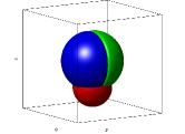
The last benchmark problem we consider is a compound droplet spreading on a solid sphere, which is more complicated and can also be used to test the present LB method in predicting the contact angle of multiphase flow in a complex geometry. The schematic of the problem is shown in Fig. 5, where a hemispherical compound droplet composed of blue ($C_{1}$) and green ($C_{2}$) fluids is initially placed on a solid sphere, and is immersed in another fluid ($C_{3}$). Under the assumption of two fluids ($C_{1}$ and $C_{2}$) with the same size, density, viscosity and surface wettability, the compound droplet would eventually form a spherical shape under the action of interfacial tensions, which can be regarded as a single-phase droplet. In this case, we can obtain the asymptotic solution of the equilibrium shape. As seen from Figs. 5 and 5, when the droplet reaches a steady state, the contact angle $\theta_{pre}$ on spherical convex surface can be given by Extrand2012

where $V_{t}=V_{0}+V_{b}$ with $V_{0}$ and $V_{b}$ being the volumes of the compound droplet and the spherical solid covered by the droplet. Actually, it is easy to obtain the initial volume $V_{0}$ as

where $R_{0}$ is the initial radius of the hemispherical droplet and $R_{s}$ is the radius of the solid sphere. If $V_{b}$ is less than the half volume of the solid sphere $V_{s}$, see Fig. 5, one can derive its expression as

On the contrary, if $V_{b}$ is larger than the half volume of the solid sphere $V_{s}$, see Fig. 5, it can be determined by

On the other hand, when the droplet is in equilibrium state with $R_{l}$, the volume of the droplet can also be given by

where $h_{1}=R_{s}(1-\cos\alpha)$ and $h_{2}=R_{l}[1-\cos(\pi-\theta_{pre}-\alpha)]$. Then one can determine the center of the steady droplet through calculating the distance $d_{O_{j}O_{s}}$,

From above analysis, we can predict the equilibrium shape of the compound droplet with the asymptotic solution. However, for a ternary-phase flow, there exits a triple point where the interfacial angles are $\varphi_{1}$, $\varphi_{2}$ and $\varphi_{3}$, and satisfy the condition $\varphi_{1}+\varphi_{2}+\varphi_{3}=2\pi$. Based on the balance of interfacial angles at the equilibrium state, one can obtain

Owing to the fact that $\varphi_{1}=\varphi_{2}\approx\pi/2$ and $\varphi_{3}\approx\pi$, which can be seen from Figs. 5 and 5, in the following simulations, we choose $\sigma_{12}=0.0025$ and $\sigma_{13}=\sigma_{23}=0.05$ to obtain $\varphi_{1}=\varphi_{2}=88.6^{\circ}$. Some other parameters are set as $\rho_{1}=\rho_{2}=10$, $\rho_{3}=1$, $R_{0}=50\delta x$, $R_{s}=25\delta x$, $m_{0}=0.01$, $\varepsilon_{0}=0.5$, $\varepsilon=5\delta x$, $\delta x=0.1$, $c=10$, $d_{0}=0.4$, $s^{f_{i}}_{0}=s^{f_{i}}_{21}=1.0$, $s^{f_{i}}_{1}=10/19$, $s^{g}_{0}=1.0$ and $s^{g}_{1}=s^{g}_{3}=s^{g}_{4}=1.2$. We perform some simulations, and present the numerical (solid curve) and asymptotic (dashed curve) solutions of the equilibrium droplet shape in Fig. 6 where the contact angles are $\theta_{1,2}=30^{\circ}$, $\theta_{1,2}=60^{\circ}$, $\theta_{1,2}=90^{\circ}$ and $\theta_{1,2}=120^{\circ}$. It is obvious that the numerical results agree well with the asymptotic solutions except for the difference at the triple point. Furthermore, Fig. 7 shows a comparison between the predicted contact angle $\theta_{pre}$ based on Eq. (34) and the specified contact angle $\theta_{1,2}$. From this figure, one can find that there is a good agreement between the numerical results and the asymptotic solutions, which illustrates that the DD-CCLB method has a good performance in the study of the multiphase flow in complex solid surface.

Unlike the static-state benchmark problems considered above, in this part, we investigate a compound droplet passing through the wavy channel, which is a typical irregular domain with a complex geometrical shape. The configuration of the problem is given in Fig. 8, where a concentric droplet composed of the red inner droplet with $R_{1}=L/5$ and the blue outer droplet with $R_{2}=L/3$ is located at $(L/2,L/2)$ of the computational domain. Besides, the top and bottom boundaries of the wavy channel are defined by $U(x)=-B(x)=0.05L\sqrt{x/L}\sin(3\pi x/L)$. To reflect the effects of different wetting boundary conditions in the DD-CC equations, we introduce two characteristic functions,

and then the characteristic function $\phi$ and the source term $\phi\mu_{C_{i}}$ appeared in the DD-CC equations can be rewritten as

and

In our simulations, a parabolic velocity with the mean velocity $u_{c}=0.003$ is imposed on the inlet and outlet of the channel, and the other parameters are fixed as $L=15$, $\rho_{1}=\rho_{2}=1.0$, $\rho_{3}=0.1$, $\sigma_{ij}=0.004$ where $i\neq j$, $m_{0}=0.01$, $\varepsilon_{0}=0.6$, $\varepsilon=8\delta x$, $\delta x=0.1$, $c=40$, $d_{0}=0.3$. We carry out some simulations, and plot the results in Fig. 9. From this figure, one can see that the compound droplet can be separated in different patterns under different wetting properties of the solid walls. For example, as shown in Fig. 9 where $\theta^{1,2}_{13}=120^{\circ}$ and $\theta^{1,2}_{23}=60^{\circ}$, the concentric droplet splits into two blue subdroplets adhered to the solid walls and an unbroken red droplet passes through the channel. In contrast, if $\theta^{1,2}_{13}=60^{\circ}$ and $\theta^{1,2}_{23}=120^{\circ}$ [see Fig. 9], the red subdroplets are adhered to the solid walls and the blue droplet can pass through the channel. For the case of $\theta^{1}_{13}=\theta^{2}_{23}=120^{\circ}$ and $\theta^{1}_{23}=\theta^{2}_{13}=60^{\circ}$ shown in Fig. 9, the red and blue droplets can be split from the concentric droplet and then adhered to the top and bottom walls, respectively.

References

- (1) D. Acosta-Soba, F. Guillén-González, and J. Rodríguez-Galván, An upwind DG scheme preserving the maximum principle for the convective Cahn-Hilliard model, Numer. Algorithms, 92 (2023), pp. 1589–1619.
- (2) S. Aland, J. Lowengrub, and A. Voigt, Two-phase flow in complex geometries: A diffuse domain approach, Comput. Model. Eng. Sci., 57 (2010), pp. 77–106.
- (3) F. Boyer and S. Minjeaud, Hierarchy of consistent n-component Cahn-Hilliard systems, Math. Models Methods Appl. Sci., 24 (2014), pp. 2885–2928.
- (4) J. Cahn and J. Hilliard, Free energy of a non-uniform system I. Interfacial free energy, J. Chem. Phys., 28 (1958), pp. 258–367.
- (5) Z. Chai and B. Shi, Multiple-relaxation-time lattice Boltzmann method for the Navier-Stokes and nonlinear convection-diffusion equations: Modeling, analysis, and elements, Phys. Rev. E, 102 (2020), p. 023306.
- (6) Z. Chai, X.Yuan, and B. Shi, Rectangular multiple-relaxation-time lattice boltzmann method for the Navier-Stokes and nonlinear convection-diffusion equations: General equilibrium and some important issues, Phys. Rev. E, 108 (2023), p. 015304.
- (7) S. Chen and G. Doolen, Lattice Boltzmann method for fluid flows, Annu. Rev. Fluid Mech., 30 (1998), pp. 329–364.
- (8) X. Chen and G. Hu, Multiphase flow in mircrofluidic devices, Adv. Appl. Mech., 45 (2015), p. 201503.
- (9) C. Coreixas, B. Chopard, and J. Latt, Comprehensive comparison of collision models in the lattice Boltzmann framework: Theoretical investigations, Phys. Rev. E, 100 (2019), p. 033305.
- (10) D. d’Humières, Multiple-relaxation-time lattice boltzmann models in three dimensions, Philos. Trans. R. Soc. London A, 360 (2002), p. 437.
- (11) S. Dong, Wall-bounded multiphase flows of N immiscible incompressible fluids: Consistency and contact-angle boundary condition, J. Comput. Phys., 338 (2017), pp. 21–67.
- (12) S. Dong, Multiphase flows of N immiscible incompressible fluids: A reduction-consistent and thermodynamically-consistent formulation and associated algorithm, J. Comput. Phys., 361 (2018), pp. 1–49.
- (13) C. Elliott and H. Garcke, On the Cahn–Hilliard equation with degenerate mobility, SIAM J. Math. Anal., 27 (1996), pp. 404–423.
- (14) C. Extrand and S. Moon, Indirect methods to measure wetting and contact angles on spherical convex and concave surfaces, Langmuir, 28 (2012), p. 7775.
- (15) H. Gan, X. Shan, T. Eriksson, B. Lok, and Y. Lam, Reduction of droplet volume by controlling actuating waveforms in inkjet printing for micro-pattern formation, J. Micromech. Microeng., 19 (2009), p. 055010.
- (16) Z. Guo, F. Yu, P. Lin, S. Wise, and J. Lowengrub, A diffuse domain method for two-phase flows with large density ratio in complex geometries, J. Fluid Mech., 907 (2021), p. A38.
- (17) Z. Huang, G. Lin, and A. M. Ardekani, Consistent, essentially conservative and balanced-force phase-field method to model incompressible two-phase flows, J. Comput. Phys., 406 (2020), p. 109192.
- (18) T. Krüeger, H. Kusumaatmaja, A. Kuzmin, O. Shardt, G. Silva, and E. M. Viggen, The Lattice Boltzmann Method: Principles and Practice, Springer, Switzerland, 2017.
- (19) W. Li, R. Vigil, I. Beresnev, P. Iassonov, and R. Ewing, Vibration-induced mobilization of trapped oil ganglia in porous media: Experimental validation of a capillary-physics mechanism, J. Colloid Interface Sci., 289 (2005), pp. 193–199.
- (20) X. Li, J. Lowengrub, A. Rätz, and A. Voigt, Solving PDEs in complex geometries: A diffuse domain approach, Commun. Math. Sci., 7 (2009), pp. 81–107.
- (21) H. Liang, J. Xu, J. Chen, Z. Chai, and B. Shi, Lattice boltzmann modeling of wall-bounded ternary fluid flows, Appl. Math. Model., 73 (2019), pp. 487–513.
- (22) X. Liu, Z. Chai, C. Zhan, B. Shi, and W. Zhang, A diffuse-domain phase-field lattice Boltzmann method for two-phase flows in complex geometries, Multiscale Model. Simul., 20 (2022), pp. 1411–1436.
- (23) J. Lowengrub and L. Truskinovsky, Quasi-incompressible Cahn-Hilliard fluids and topological transitions, R. Soc. Lond. Proc. Ser. A Math. Phys. Eng. Sci., 454 (1998), pp. 2617–2654.
- (24) J. Shen, Modeling and numerical approximation of two-phase incompressible flows by a phase-field approach, Multiscale Modeling and Analysis for Materials Simulation, Lect. Notes Ser. Inst. Math. Sci. Natl. Univ. Singap. 22, 2011.
- (25) S. Succi, The Lattice Boltzmann Equation for Fluid Dynamics and Beyond, Oxford: Clarendon Press, 2001.
- (26) Q. Xia, J. Kim, and Y. Li, Modeling and simulation of multi-component immiscible flows based on a modified Cahn-Hilliard equation, Eur. J. Mech. B, Fluids, 97 (2022), pp. 194–204.
- (27) J. Yang, Y. Li, and J. Kim, Modified multi-phase diffuse-interface model for compound droplets in contact with solid, J. Comput. Phys., 491 (2023), p. 112345.
- (28) J. Yang, Z. Tan, J. Wang, and J. Kim, Modified diffuse interface fluid model and its consistent energy-stable computation in arbitrary domains, J. Comput. Phys., 488 (2023), p. 112216.
- (29) F. Yu, Z. Guo, and J. Lowengrub, Higher-order accurate diffuse-domain methods for partial differential equations with dirichlet boundary conditions in complex, evolving geometries, J. Comput. Phys., 406 (2020), p. 109174.
- (30) C. Zhang, H. Ding, P. Gao, and Y. Wu, Diffuse interface simulation of ternary fluids in contact with solid, J. Comput. Phys., 309 (2016), pp. 37–51.