\stackMath

A consistence-stability approach to hydrodynamic limit of interacting particle systems on lattices

Angeliki Menegaki Institut des hautes études Scientifiques, 35 Rte de Chartres, 91440, Bures-sur-Yvette, France [email protected] and Clément Mouhot DPMMS, University of Cambridge, Wilberforce Road, Cambridge CB3 0WA, UK [email protected]

Abstract.

This is a review based on the presentation done at the seminar Laurent Schwartz in December $2021$ . It is announcing results in the forthcoming [MMM22]. This work presents a new simple quantitative method for proving the hydrodynamic limit of a class of interacting particle systems on lattices. We present here this method in a simplified setting, for the zero-range process and the Ginzburg-Landau process with Kawasaki dynamics, in the parabolic scaling and in dimension $1$ . The rate of convergence is quantitative and uniform in time. The proof relies on a consistence-stability approach in Wasserstein distance, and it avoids the use of the “block estimates”.

1. The general method

We consider the hydrodynamic limit of interacting particle systems on a lattice. The problem is to show that under an appropriate scaling of time and space, the local particle densities of a stochastic lattice gas converge to the solution of a macroscopic partial differential equation. We first present our method abstractly and then sketch applications to two concrete models: the zero-range process (ZRP) and the Ginzburg Landau process with Kawasaki dynamics (GLK). The hydrodynamic limit is known at a qualitative level for all these models under both hyperbolic and parabolic scalings for the ZRP and under parabolic scaling for the GLK, see [GPV88, Yau91, Rez91, KL99]. However finding quantitative error estimates had remained an important opened question, as well as understanding the long-time behaviour of the hydrodynamic limit. First results towards quantitative error, in the particular case of the Ginzburg-Landau process with Kawasaki dynamics in dimension $1$ , were obtained in the two-parts work [DMOWa, DMOWb], which builds upon partial progresses in [GOVW09].

1.1. Set up and notation

We denote by $\mathsf{X}$ the state space at a given site (number of particles, spin, etc.), which will in this paper be $\mathbb{N}$ (ZRP) or $\mathbb{R}$ (GLK). Consider the discrete torus $\mathbb{T}_{N}^{d}$ and the corresponding phase space of particle configurations $\mathsf{X}_{N}:=\mathsf{X}^{\mathbb{T}^{d}_{N}}$ . Variables in $\mathbb{T}^{d}_{N}$ are called microscopic and denoted by $x,y,z$ , whereas variables in the limit continuous torus $\mathbb{T}^{d}$ are called macroscopic and denoted by $u$ ; finally particle configurations in $\mathsf{X}_{N}$ are denoted by $\eta$ . The canonical embeddding $\mathbb{T}_{N}^{d}\to\mathbb{T}^{d}$ , $x\mapsto\frac{x}{N}$ means the macroscopic distance between sites of the lattice is $\frac{1}{N}$ . Given a particle configuration $\eta\in\mathsf{X}_{N}$ , we define the empirical measure

(1.1)

\alpha_{\eta}^{N}:=\mathop{\mathchoice{\stackon[-3.8ex]{\displaystyle\sum}{\smash{\rule{0.4pt}{17.22217pt}}}}{\stackon[-2.6ex]{\textstyle\sum}{\smash{\rule{0.4pt}{12.48604pt}}}}{\stackon[-1.9ex]{\scriptstyle\sum}{\smash{\rule{0.4pt}{9.47217pt}}}}{\stackon[-1.4ex]{\scriptscriptstyle\sum}{\smash{\rule{0.4pt}{7.3194pt}}}}}_{x\in\mathbb{T}^{d}_{N}}\eta_{x}\delta_{\frac{x}{N}}\in\mathcal{M}_{+}(\mathbb{T}^{d}).

where $\eta_{x}$ denotes the value of $\eta$ at $x\in\mathbb{T}^{d}_{N}$ , and $\mathcal{M}_{+}(\mathbb{T}^{d})$ is the space of positive Radon measures on the torus, and $\mathop{\mathchoice{\stackon[-3.8ex]{\displaystyle\sum}{\smash{\rule{0.4pt}{17.22217pt}}}}{\stackon[-2.6ex]{\textstyle\sum}{\smash{\rule{0.4pt}{12.48604pt}}}}{\stackon[-1.9ex]{\scriptstyle\sum}{\smash{\rule{0.4pt}{9.47217pt}}}}{\stackon[-1.4ex]{\scriptscriptstyle\sum}{\smash{\rule{0.4pt}{7.3194pt}}}}}$ denotes the “average sum”, here $N^{-d}\sum_{x\in\mathbb{T}^{d}_{N}}$ .

At the microscopic level, the interacting particle system evolves through a stochastic process and the time-dependent probability measure describing the law of $\eta$ is denoted by $\mu_{t}^{N}\in P(\mathsf{X}_{N})$ . We consider a linear operator $\mathcal{L}_{N}:C_{b}(\mathsf{X}_{N})\rightarrow C_{b}(\mathsf{X}_{N})$ generating uniquely a Feller semigroup $e^{t\mathcal{L}_{N}}$ on $P(\mathsf{X}_{N})$ (see [Lig85, Chapter 1]) so that given $\mu_{0}^{N}\in P(\mathsf{X}_{N})$ the solution $\mu_{t}^{N}=e^{t\mathcal{L}_{N}}\mu^{N}_{0}\in P(\mathsf{X}_{N})$ satisfies

(1.2)

\forall\,\Phi\in C_{b}(\mathsf{X}_{N}),\quad\frac{{\rm d}}{{\rm d}t}\langle\Phi,\mu^{N}_{t}\rangle=\langle\mathcal{L}_{N}\Phi,\mu^{N}_{t}\rangle,

where $C_{b}(\mathsf{X}_{N})$ denotes continuous bounded real-valued functions and $\langle\cdot,\cdot\rangle$ denotes the duality bracket between $C_{b}(\mathsf{X}_{N})$ and $P(\mathsf{X}_{N})$ .

At the macroscopic level, we consider a map $\mathcal{L}_{\infty}:\mathcal{M}_{+}(\mathbb{G}_{\infty})\rightarrow\mathcal{M}_{+}(\mathbb{G}_{\infty})$ (in general unbounded and nonlinear) and the evolution problem

(1.3)

\partial_{t}f_{t}=\mathcal{L}_{\infty}f_{t},\quad f_{t=0}=f_{0}.

A measure $\mu^{N}\in P(\mathsf{X}_{N})$ is called invariant for (1.2) if

\forall\,\Phi\in C_{b}(\mathsf{X}_{N}),\quad\big{\langle}\mu^{N},\mathcal{L}_{N}\Phi\big{\rangle}=0.

We also denote $\operatorname{Lip}(\mathsf{X}_{N})$ the Lipschitz functions $\Phi:\mathsf{X}_{N}\to\mathbb{R}$ with respect to the (normalised) $\ell^{1}$ norm: for every $\eta,\zeta\in\mathsf{X}_{N}$ , $|\Phi(\eta)-\Phi(\zeta)|\leq C_{\Phi}\mathop{\mathchoice{\stackon[-3.8ex]{\displaystyle\sum}{\smash{\rule{0.4pt}{17.22217pt}}}}{\stackon[-2.6ex]{\textstyle\sum}{\smash{\rule{0.4pt}{12.48604pt}}}}{\stackon[-1.9ex]{\scriptstyle\sum}{\smash{\rule{0.4pt}{9.47217pt}}}}{\stackon[-1.4ex]{\scriptscriptstyle\sum}{\smash{\rule{0.4pt}{7.3194pt}}}}}_{x\in\mathbb{T}_{N}^{d}}|\eta_{x}-\zeta_{x}|$ , and we denote the smallest such constant $C_{\Phi}$ by $[\Phi]_{\operatorname{Lip}(\mathsf{X}_{N})}\in\mathbb{R}_{+}$ .

1.2. Abstract assumptions

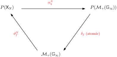
We make the following assumptions on (1.2)-(1.3):

(H0) Local equilibrium structure. There are $n_{\lambda}:\text{Conv}(\mathsf{X})\to\mathbb{R}_{+}$ depending on $\lambda\in\mathbb{R}$ (Conv denotes the convex hull) and $\sigma:\text{Conv}(\mathsf{X})\to\mathbb{R}$ so that: (i) $n_{\lambda}^{\otimes\mathbb{T}^{d}_{N}}$ is invariant on $\mathsf{X}_{N}$ for each $\lambda$ , and (ii) for any $\rho\in\text{Conv}(\mathsf{X})$ , $\mathbb{E}_{n_{\sigma(\rho)}}[\eta_{x}]=\rho$ . We then define, given a macroscopic profile $f$ on $\mathbb{T}^{d}$ , the local Gibbs measure

\vartheta^{N}_{f}(\eta):=\nu_{\sigma\left(f\left(\frac{\cdot}{N}\right)\right)}^{N}(\eta)\quad\text{where}\quad\nu_{F}^{N}(\eta):=\prod_{x\in\mathbb{G}_{N}}n_{F(x)}(\eta(x)).

The two maps $\eta\mapsto\alpha_{\eta}^{N}$ and $f\mapsto\vartheta^{N}_{f}$ allow comparisons between the microscopic and macroscopic scales, as summarized in Figure 1.

Refer to caption — Figure 1. The functional setting.

(H1) Microscopic stability. The semigroup $e^{t\mathcal{L}_{N}}$ satisfies

(1.4)

\displaystyle\forall\,\Phi\in\operatorname{Lip}(\mathsf{X}_{N}),\quad\left[e^{t\mathcal{L}_{N}}\Phi\right]_{\operatorname{Lip}(\mathsf{X}_{N})}\leq\left[\Phi\right]_{\operatorname{Lip}(\mathsf{X}_{N})}.

(H2) Macroscopic stability. There is a Banach space $\mathfrak{B}\subset\mathcal{M}_{+}(\mathbb{G}_{\infty})$ so that (1.3) is locally well-posed in $\mathfrak{B}$ ; given the maximal time of existence $T_{m}\in(0,+\infty]$ we denote for $t\in[0,T_{m})$ , $R(t):=\left\|f_{t}-f_{\infty}\right\|_{\mathfrak{B}}$ when (1.3) has a unique stationary solution $f_{\infty}\in\mathfrak{B}$ with mass $\int_{\mathbb{T}^{d}}f_{\infty}=\int_{\mathbb{T}^{d}}f_{0}$ , otherwise we denote $R(t):=\left\|f_{t}\right\|_{\mathfrak{B}}$ .

(H3) Consistency. There is a consistency error $\epsilon(N)\to 0$ as $N\to\infty$ so that for $T\in[0,T_{m})$

\frac{1}{T}\int_{0}^{T}\int_{0}^{t}\left\langle\left(e^{(t-s)\mathcal{L}_{N}}\Phi\right),\left[\mathcal{L}_{N}^{*}\left(\frac{{\rm d}\vartheta_{f_{s}}^{N}}{{\rm d}\nu^{N}_{\infty}}\right)-\frac{{\rm d}}{{\rm d}s}\left(\frac{{\rm d}\vartheta_{f_{s}}^{N}}{{\rm d}\nu^{N}_{\infty}}\right)\right]{\rm d}\nu^{N}_{\infty}\right\rangle\,{\rm d}s\,{\rm d}t\leq\epsilon(N)[\Phi]_{\operatorname{Lip}(\mathsf{X}_{N})}\int_{0}^{t}R(s)\,{\rm d}s

for any $\Phi\in\operatorname{Lip}(\mathsf{X}_{N})$ , where $\nu^{N}_{\infty}$ is an equilibrium measure.

1.3. The abstract strategy

Theorem 1.1.

Consider (1.2)-(1.3) with the assumptions (H0)–(H1)–(H2)–(H3). Let $\phi\in C^{\infty}(\mathbb{T}^{d})$ , $\mu_{0}^{N}\in P_{1}(X_{N})$ for all $N\geq 1$ , $f_{0}\in\mathcal{B}$ . Then

(1.5)

\forall\,T\in[0,T_{m}),\quad\frac{1}{T}\int_{0}^{T}\left\|\mu_{t}^{N}-\vartheta_{f_{t}}^{N}\right\|_{\operatorname{Lip}^{*}}\,{\rm d}t\lesssim\epsilon(N)\int_{0}^{T}R(s)\,{\rm d}s+\left\|\mu_{0}^{N}-\vartheta_{f_{0}}^{N}\right\|_{\operatorname{Lip}^{*}}.

Remark 1.

Note that $\|\mu_{t}^{N}-\vartheta_{f_{t}}^{N}\|_{\operatorname{Lip}^{*}}\to 0$ as $N\to\infty$ implies that the empirical measure (1.1) sampled from the law $\mu^{N}_{t}$ satisfies

(1.6)

\forall\,\phi\in C_{b}(\mathbb{G}),\ \forall\,\epsilon>0,\ \forall\,t\geq 0,\quad\lim_{N\rightarrow\infty}\mu^{N}_{t}\left(\left\{|\langle\alpha^{N}_{\eta},\varphi\rangle-\langle f_{t},\varphi\rangle|>\epsilon\right\}\right)=0

with a rate of convergence (thus recovering quantitatively results from [GPV88]):

	$\displaystyle\mu^{N}_{t}\left(\left\{\|\langle\alpha^{N}_{\eta},\varphi\rangle-\langle f_{t},\varphi\rangle\|>\epsilon\right\}\right)$
	$\displaystyle\leq\mu^{N}_{t}\left(\left\{\langle\alpha^{N}_{\eta},\varphi\rangle\geq\langle f_{t},\varphi\rangle+\epsilon\right\}\right)+\mu^{N}_{t}\left(\left\{\langle\alpha^{N}_{\eta},\varphi\rangle\leq\langle f_{t},\varphi\rangle-\epsilon\right\}\right)$
	$\displaystyle\leq\int_{\mathsf{X}_{N}}\left[F_{\epsilon}^{+}\left(\left\langle\phi,\alpha_{\eta}^{N}\right\rangle\right)-F_{\epsilon}^{+}\left(\left\langle\phi,f_{t}\right\rangle\right)\right]\,{\rm d}\mu_{t}^{N}+\int_{\mathsf{X}_{N}}\left[F_{\epsilon}^{-}\left(\left\langle\phi,\alpha_{\eta}^{N}\right\rangle\right)-F^{-}_{\epsilon}\left(\left\langle\phi,f_{t}\right\rangle\right)\right]\,{\rm d}\mu_{t}^{N}$

where $F_{\epsilon}^{\pm}$ are mollified version of the characteristic functions of respectively $\{z\geq\left\langle\phi,f_{t}\right\rangle+\epsilon\}$ and $\{z\leq\left\langle\phi,f_{t}\right\rangle-\epsilon\}$ , which yields

\sup_{t\in[0,T]}\mu^{N}_{t}\left(\left\{|\langle\alpha^{N}_{\eta},\varphi\rangle-\langle f_{t},\varphi\rangle|>\epsilon\right\}\right)\lesssim\epsilon^{-1}\|\mu_{t}^{N}-\vartheta_{f_{t}}^{N}\|_{\operatorname{Lip}^{*}}+\epsilon^{-2}N^{-d}.

2. Concrete applications

We apply the abstract result to two archetypical models, the zero-range process (ZRP), and the Ginzburg-Landau process with Kawasaki dynamics (GLK).

2.1. The ZRP

In this case, the state space at each site is $\mathsf{X}=\mathbb{N}$ . Given the choice of a transition function $p\in P(\mathbb{T}^{d}_{N})$ with $p(0)=0$ and a jump rate function $g:\mathbb{N}\rightarrow\mathbb{R}_{+}$ , the base generator $\hat{\mathcal{L}}_{N}$ writes

(2.1)

\forall\,\Phi\in C_{b}(\mathsf{X}_{N}),\ \forall\,\eta\in\mathsf{X}_{N},\quad\hat{\mathcal{L}}_{N}\Phi(\eta):=\sum_{x,y\in\mathbb{T}^{d}_{N}}p(y-x)g(\eta_{x})\left[\Phi(\eta^{xy})-\Phi(\eta)\right]

where $\eta^{xy}$ is defined as before. The local equilibrium structure of (H0) is given by

(2.2)			$\displaystyle n_{\lambda}(k):=\frac{\lambda^{k}}{g(k)!Z(\lambda)}\quad\text{ with }\quad Z(\lambda):=\sum_{k=0}^{+\infty}\frac{\lambda^{k}}{g(k)!}$
(2.3)			$\displaystyle\sigma\ \text{ is defined implicitely by }\ \sigma(\rho)\frac{Z^{\prime}(\sigma(\rho))}{Z(\sigma(\rho))}\equiv\rho$

denoting $g(k)!:=g(k)g(k-1)\cdots g(1)$ . The pair $(g,\sigma)$ thus constructed satisfies $\mathbb{E}_{n_{\sigma(\alpha)}}[g]=\sigma(\alpha)$ . When $f\equiv\rho\in[0,+\infty)$ is constant, the local Gibbs measure $\vartheta_{\rho}^{N}=\nu_{\sigma(\rho)}^{N}$ is invariant with average number of particles $\rho$ . The mean transition rate is defined by $\gamma:=\sum_{x\in\mathbb{Z}^{d}}xp(x)\in\mathbb{R}^{d}$ . When $\gamma\not=0$ , the first non-zero asymptotic dynamics as $N\to\infty$ is given by the hyperbolic scaling $\mathcal{L}_{N}:=N\hat{\mathcal{L}}_{N}$ , and the corresponding expected limit equation is $\partial_{t}f=\gamma\cdot\nabla[\sigma(f)]$ . When $\gamma=0$ , the first non-zero asymptotic dynamics as $N\to\infty$ is the given by the parabolic scaling $\mathcal{L}_{N}:=N^{2}\hat{\mathcal{L}}_{N}$ , and the corresponding limit equation is formally

(2.4)

\partial_{t}f=\Delta_{a}[\sigma(f)]\quad\text{ with }\quad\Delta_{a}:=\sum_{i,j=1}^{d}a_{ij}\partial^{2}_{ij}\quad\text{and}\quad a_{ij}:=\sum_{x\in\mathbb{Z}^{d}}p(x)x_{i}x_{j}.

We make the following assumptions on the jump rate function $g:\mathbb{N}\rightarrow[0,\infty)$ .

(HZRP) The jump rate $g$ satisfies $g(0)=0$ , $g(n)>0$ for all $n>0$ , is non-decreasing, uniformly Lipschitz $\sup_{n\geq 0}|g(n+1)-g(n)|<+\infty$ , and there are $n_{0}>0$ and $\beta>0$ such that $g(n^{\prime})-g(n)\geq\beta$ for any $n^{\prime}\geq n+n_{0}$ .

The main result on the ZRP is:

Theorem 2.1 (Hydrodynamic limit for the ZRP).

Consider $\hat{\mathcal{L}}_{N}$ defined in (2.1) with $g$ satisfying (HZRP). Let $d=1$ , $f_{0}\in C^{3}(\mathbb{T})$ with $f_{0}\geq\delta>0$ , and $\mu_{0}^{N}\in P_{1}(\mathsf{X}_{N})$ for all $N\geq 1$ . Assume $\gamma=0$ , define $\mu^{N}_{t}=e^{tN^{2}\hat{\mathcal{L}}_{N}}$ and $f_{t}\in C([0,T),C^{3}(\mathbb{T}^{d}))$ solution to (2.4), then the following convergence holds (with quantitative constants)

(2.5)

\sup_{T\geq 0}\frac{1}{T}\int_{0}^{T}\left\|\mu_{t}^{N}-\vartheta_{f_{t}}^{N}\right\|_{\operatorname{Lip}^{*}}\,{\rm d}t\lesssim N^{-\frac{1}{8}}+\left\|\mu_{0}^{N}-\vartheta_{f_{0}}^{N}\right\|_{\operatorname{Lip}^{*}}.

2.2. The GLK

In this case, the state space at each site is $\mathsf{X}=\mathbb{R}$ . Given the choice of a single-site potential $V\in C^{2}(\mathbb{R})$ , the base generator $\hat{\mathcal{L}}_{N}$ writes

(2.6)

\hat{\mathcal{L}}_{N}\Phi(\eta):=\frac{1}{2}\sum_{x\sim y\in\mathbb{T}^{d}_{N}}\left(\frac{\partial}{\partial\eta_{x}}-\frac{\partial}{\partial\eta_{y}}\right)^{2}-\frac{1}{2}\sum_{x\sim y\in\mathbb{T}^{d}_{N}}\left[V^{\prime}(\eta_{x})-V^{\prime}(\eta_{y})\right]\left(\frac{\partial}{\partial\eta_{x}}-\frac{\partial}{\partial\eta_{y}}\right)

where $x\sim y$ denotes neighbouring sites. The local equilibrium structure is given by

	$\displaystyle n_{\lambda}(r):=\frac{e^{\lambda r-V(r)}}{Z(\lambda)}\quad\text{ with }\quad Z(\lambda):=\int_{\mathbb{R}}e^{\lambda r-V(r)}\,{\rm d}r$
	$\displaystyle\sigma\ \text{ is defined implicitely by }\ \frac{Z^{\prime}(\sigma(\rho))}{Z(\sigma(\rho))}\equiv\rho.$

When $f\equiv\rho\in\mathbb{R}$ is constant, the local Gibbs measure $\vartheta_{\rho}^{N}=\nu_{\sigma(\rho)}^{N}$ is invariant with average spin $\rho$ . The hyperbolic scaling formally leads to zero and the parabolic scaling $\mathcal{L}_{N}:=N^{2}\hat{\mathcal{L}}_{N}$ formally leads to

(2.7)

\partial_{t}f=2\Delta[\sigma(f)].

We assume that the single-site potential satisfies

(HGLK) The potential $V$ is $C^{2}$ and decomposes as $V(u)=V_{0}(u)+V_{1}(u)$ with $V_{0}^{\prime\prime}(u)\geq\kappa$ for all $u\in\mathbb{R}$ for some $\kappa>0$ and $\|V_{1}\|_{W^{1,\infty}(\mathbb{R})}\lesssim 1$ .

This assumption is similar with those in [GOVW09, DMOWa, Fat13]. One can take for example a double-well potential, provided it is uniformly convex at infinity.

Theorem 2.2 (Hydrodynamic limit for the GLK).

Consider $\mathcal{L}_{N}$ defined in (2.6) with $V$ satisfying (HGLK). Let $d=1$ , $f_{0}\in C^{3}(\mathbb{T}^{d})$ and $\mu_{0}^{N}\in P_{1}(\mathsf{X}_{N})$ for all $N\geq 1$ . Define $\mu^{N}_{t}=e^{tN^{2}\hat{\mathcal{L}}_{N}}$ and $f_{t}\in C([0,+\infty),C^{3}(\mathbb{T}^{d}))$ the global solution to (2.7), then the following convergence holds (with quantitative constants)

(2.8)

\sup_{T\geq 0}\frac{1}{T}\int_{0}^{T}\left\|\mu_{t}^{N}-\vartheta_{f_{t}}^{N}\right\|_{\operatorname{Lip}^{*}}\,{\rm d}t\lesssim N^{-\frac{1}{8}}+\left\|\mu_{0}^{N}-\vartheta_{f_{0}}^{N}\right\|_{\operatorname{Lip}^{*}}.

3. The abstract strategy

In this section we sketch the proof of Theorem 1.1. Let $f_{t}$ be a solution to (1.3). Given $0<\ell<N$ , we denote by $\eta^{\ell}$ for the local $\ell$ -average $\eta^{\ell}_{x}:=\mathop{\mathchoice{\stackon[-3.8ex]{\displaystyle\sum}{\smash{\rule{0.4pt}{17.22217pt}}}}{\stackon[-2.6ex]{\textstyle\sum}{\smash{\rule{0.4pt}{12.48604pt}}}}{\stackon[-1.9ex]{\scriptstyle\sum}{\smash{\rule{0.4pt}{9.47217pt}}}}{\stackon[-1.4ex]{\scriptscriptstyle\sum}{\smash{\rule{0.4pt}{7.3194pt}}}}}_{|y-x|\leq\ell}\eta_{y}$ .

Denote by $F^{N}_{t}:=\frac{{\rm d}\mu^{N}_{t}}{{\rm d}\nu^{N}_{\infty}}$ and $G^{N}_{t}:=\frac{{\rm d}\vartheta^{N}_{f_{t}}}{{\rm d}\nu^{N}_{\infty}}$ the densities with respect to $\nu^{N}_{\infty}$ , and write

\displaystyle\frac{\,{\rm d}}{\,{\rm d}t}\Big{(}F^{N}_{t}-G_{t}^{N}\Big{)}=\mathcal{L}_{N}^{*}\Big{(}F^{N}_{t}-G_{t}^{N}\Big{)}+\left(\mathcal{L}_{N}^{*}G_{t}^{N}-\partial_{t}G_{t}^{N}\right)

so that Duhamel’s formula yields

\displaystyle F^{N}_{t}-G_{t}^{N}=e^{t\mathcal{L}_{N}^{*}}\left(F^{N}_{0}-G_{0}^{N}\right)+\int_{0}^{t}e^{(t-s)\mathcal{L}_{N}^{*}}\left(\mathcal{L}_{N}^{*}G_{s}^{N}-\partial_{s}G_{s}^{N}\right)\,{\rm d}s.

Take $\Phi\in\operatorname{Lip}(\mathsf{X}_{N})$ with $\|\Phi\|_{\operatorname{Lip}(\mathsf{X}_{N})}\leq 1$ and integrate the above equation to get

	$\displaystyle\int_{\mathsf{X}_{N}}\Phi\Big{(}F^{N}_{t}-G_{t}^{N}\Big{)}\,{\rm d}\nu^{N}_{\infty}$
	$\displaystyle=\underbrace{\int_{\mathsf{X}_{N}}\left(e^{t\mathcal{L}_{N}}\Phi\right)\Big{(}F^{N}_{0}-G_{0}^{N}\Big{)}\,{\rm d}\nu^{N}_{\infty}}_{I_{1}(t)}+\underbrace{\int_{\mathsf{X}_{N}}\int_{0}^{t}\left(e^{(t-s)\mathcal{L}_{N}}\Phi\right)\left(\mathcal{L}_{N}G_{s}^{N}-\partial_{s}G_{s}^{N}\right)\,{\rm d}\nu^{N}_{\infty}\,{\rm d}s}_{I_{2}(t)}.$

(H1) implies $I_{1}(t)\lesssim\|\mu^{N}_{0}-\vartheta_{f_{0}}^{N}\|_{\operatorname{Lip}^{*}}$ and (H3) implies $\frac{1}{T}\int_{0}^{T}I_{2}(t)\,{\rm d}t\leq\epsilon(N)\int_{0}^{T}R(s)\,{\rm d}s$ , which implies the conclusion of Theorem 1.1.

4. Proof for the ZRP

In this section we prove Theorem 2.1) (hydrodynamical limit for the ZRP). Note for this model $\mathcal{L}_{N}=\mathcal{L}_{N}^{*}$ is symmetric with respect to equilibrium measures.

Given $f_{t}\in C^{3}(\mathbb{T}^{d})$ with $f>\delta$ , $\delta>0$ , and $\rho:=\int_{\mathbb{T}^{d}}f$ , the density of the local Gibbs measure relatively to the invariant measure with mass $\rho$ is:

(4.1)

G_{t}^{N}(\eta):=\frac{{\rm d}\vartheta_{f}^{N}(\eta)}{{\rm d}\vartheta_{\rho}^{N}(\eta)}=\prod_{x\in\mathbb{T}^{d}_{N}}\left(\frac{\sigma\left(f_{t}\left(\frac{x}{N}\right)\right)}{\sigma(\rho)}\right)^{\eta(x)}\left(\frac{Z(\sigma\left(f_{t}\left(\frac{x}{N}\right)\right))}{Z(\sigma(\rho))}\right)^{-1}.

where the function $\sigma(r)$ is defined by $\langle n_{\sigma(r)},\eta(x)\rangle=r$ and the partition function $Z:[0,\lambda^{\ast})\rightarrow\mathbb{R}$ is defined in (2.2), with $\lambda^{*}\in[0,+\infty]$ denoting the radius of convergence of the series.

It is proved in [KL99, Chapter 2, Section 3] that assumption (HZRP) on $g$ implies that $\sigma=R^{-1}:[0,\infty)\rightarrow[0,\infty)$ is well-defined and strictly increasing, with

R(\lambda)=\lambda\partial_{\lambda}\log(Z(\lambda))=\frac{1}{Z(\lambda)}\sum_{n\geq 0}\frac{n\lambda^{n}}{g(n)!}.

Then the building block $n_{\rho}$ of the Gibbs measure satisfies $\langle n_{\sigma(\rho)},g(\eta(x))\rangle=\sigma(\rho)$ . Moreover (HZRP) implies that the function $\sigma$ is $C^{\infty}$ with uniform bound on all derivatives on $\mathbb{R}_{+}$ , with Lipschitz constant less than $g^{\ast}$ , and with $\inf_{\lambda>0}\lambda^{-1}\sigma(\lambda)>0$ (in particular $\sigma^{\prime}(0)>0$ ), and that the invariant measure has exponential moment bounds, see [KL99, Corollary 3.6].

4.1. Microscopic Stability – (H1)

We use the coupling of [Lig85, Rez91]. Let

(4.2)

\begin{split}\widetilde{\mathcal{L}}_{N}\Psi(\eta,\zeta):=&\sum_{x,y\in\mathbb{T}^{d}_{N}}p(y-x)\Big{(}g(\eta_{x})\wedge g(\zeta_{x})\Big{)}\Big{[}\Psi(\eta^{xy},\zeta^{xy})-\Psi(\eta,\zeta)\Big{]}\\ &+\sum_{x,y\in\mathbb{T}^{d}_{N}}p(y-x)\Big{(}g(\eta_{x})-g(\eta_{x})\wedge g(\zeta_{x})\Big{)}\Big{[}\Psi(\eta^{xy},\zeta)-\Psi(\eta,\zeta)\Big{]}\\ &+\sum_{x,y\in\mathbb{T}^{d}_{N}}p(y-x)\Big{(}g(\zeta_{x})-g(\eta_{x})\wedge g(\zeta_{x})\Big{)}\Big{[}\Psi(\eta,\zeta^{xy})-\Psi(\eta,\zeta)\Big{]}.\end{split}

for a two-variable test function $\Psi(\eta,\zeta)$ . Then $\widetilde{\mathcal{L}}_{N}\Phi(\eta)=\hat{\mathcal{L}}_{N}\Phi(\eta)$ and $\widetilde{\mathcal{L}}_{N}\Phi(\zeta)=\hat{\mathcal{L}}_{N}\Phi(\zeta)$ , and (H1) follows from the fact that $e^{t\widetilde{\mathcal{L}}_{N}}$ preserves sign and the inequality

\widetilde{\mathcal{L}}_{N}\left(\sum_{z\in\mathbb{T}^{d}_{N}}|\eta_{z}-\zeta_{z}|\right)\leq 0.

To prove the latter inequality, we compute

	$\displaystyle\widetilde{\mathcal{L}}_{N}\left(\sum_{z\in\mathbb{T}^{d}_{N}}\|\eta_{z}-\zeta_{z}\|\right)$	$\displaystyle=\sum_{x,y\in\mathbb{T}^{d}_{N}}p(y-x)\Big{(}g(\eta_{x})-g(\eta_{x})\wedge g(\zeta_{x})\Big{)}$
		$\displaystyle\hskip 56.9055pt\times\Big{[}\|\eta^{xy}_{x}-\zeta_{x}\|+\|\eta^{xy}_{y}-\zeta_{y}\|-\|\eta_{x}-\zeta_{x}\|-\|\eta_{y}-\zeta_{y}\|\Big{]}$
		$\displaystyle\quad+\sum_{x,y\in\mathbb{T}^{d}_{N}}p(y-x)\Big{(}g(\zeta_{x})-g(\eta_{x})\wedge g(\zeta_{x})\Big{)}$
		$\displaystyle\hskip 56.9055pt\times\Big{[}\|\eta_{x}-\zeta^{xy}_{x}\|+\|\eta_{y}-\zeta^{xy}_{y}\|-\|\eta_{x}-\zeta_{x}\|-\|\eta_{y}-\zeta_{y}\|\Big{]}.$

When $g(\eta_{x})-g(\eta_{x})\wedge g(\zeta_{x})>0$ necessarily $\eta_{x}-\zeta_{y}\geq 1$ and

\Big{[}|\eta^{xy}_{x}-\zeta_{x}|+|\eta^{xy}_{y}-\zeta_{y}|-|\eta_{x}-\zeta_{x}|-|\eta_{y}-\zeta_{y}|\Big{]}\leq 0.

When $g(\zeta_{x})-g(\eta_{x})\wedge g(\zeta_{x})>0$ necessarily $\zeta_{x}-\eta_{x}\geq 1$ and

\Big{[}|\eta_{x}-\zeta^{xy}_{x}|+|\eta_{y}-\zeta^{xy}_{y}|-|\eta_{x}-\zeta_{x}|-|\eta_{y}-\zeta_{y}|\Big{]}\leq 0.

4.2. Macroscopic stability – (H2)

In the parabolic scaling the limit PDE is the nonlinear diffusion equation (2.4). We take $\mathcal{B}=C^{3}$ with its standard infinity Banach norm. The proof that this norm remains uniformly bounded in time is classical in dimension $d=1$ (using the bounds on $\sigma$ ), and $f_{t}\in[\delta,1-\delta]$ for all times by maximal principle. Moreover $f_{t}\to\rho$ exponentially fast as $t\to\infty$ in $\mathcal{B}$ .

4.3. Consistency estimate – (H3)

Let $\gamma=0$ and the dimension $d=1$ .

Proposition 4.1.

Given the solution $f_{t}\in C^{3}(\mathbb{T}^{d})$ to (2.4) with $f\geq\delta$ , $\delta>0$ , and $\rho:=\int_{\mathbb{T}^{d}}f$ , and $G_{t}^{N}$ defined in (4.1), we have for every $\Phi\in\operatorname{Lip}(\mathsf{X}_{N})$ with $[\Phi]_{\operatorname{Lip}(\mathsf{X}_{N})}\leq 1$

\displaystyle\frac{1}{T}\int_{0}^{T}I_{t}^{N}\,{\rm d}t:=\frac{1}{T}\int_{0}^{T}\int_{0}^{t}\left\langle\left(e^{(t-s)\mathcal{L}_{N}}\Phi\right),\left[\mathcal{L}_{N}G^{N}_{s}-\frac{{\rm d}}{{\rm d}s}G^{N}_{s}\right]{\rm d}\nu^{N}_{\infty}\right\rangle\,{\rm d}s\,{\rm d}t=\mathcal{O}\left(N^{-\frac{1}{8}}\right)

where the constant depends on the estimates in (H2).

Proof.

We start by computing

\mathcal{L}_{N}G^{N}_{s}-\frac{{\rm d}}{{\rm d}s}G^{N}_{s}=\sum_{x\in\mathbb{T}^{d}_{N}}A_{x}^{N}G^{N}_{s}

with (note that $f_{t}\to\rho$ exponentially fast)

	$\displaystyle A_{x}^{N}$	$\displaystyle:=N^{2}\sum_{y\in\mathbb{T}^{d}_{N}}p(y-x)g(\eta_{x})\left(\frac{\sigma\left(f_{t}\left(\frac{y}{N}\right)\right)}{\sigma\left(f_{t}\left(\frac{x}{N}\right)\right)}-1\right)-\eta_{x}\frac{\sigma^{\prime}\left(f_{t}\left(\frac{x}{N}\right)\right)}{\sigma\left(f_{t}\left(\frac{x}{N}\right)\right)}\Delta_{a}[\sigma(f)]\left(\frac{x}{N}\right)$
		$\displaystyle=\frac{g(\eta_{x})}{\sigma\left(f_{t}\left(\frac{x}{N}\right)\right)}\Delta_{a}[\sigma(f)]\left(\frac{x}{N}\right)-\eta_{x}\frac{\sigma^{\prime}\left(f_{t}\left(\frac{x}{N}\right)\right)}{\sigma\left(f_{t}\left(\frac{x}{N}\right)\right)}\Delta_{a}[\sigma(f)]\left(\frac{x}{N}\right)+\mathcal{O}\left(\frac{e^{-Cs}}{N}\right)$

for some $C>0$ . Since (conservation of mass)

\int_{\mathsf{X}_{N}}\left(\sum_{x\in\mathbb{T}^{d}_{N}}A_{x}^{N}G^{N}_{s}\right)\,{\rm d}\nu_{\infty}^{N}=\int_{\mathsf{X}_{N}}\left(\sum_{x\in\mathbb{T}^{d}_{N}}A_{x}^{N}\right)\,{\rm d}\vartheta_{f_{s}}^{N}=0,

we can replace $\Phi_{t-s}:=e^{(t-s)\mathcal{L}_{N}}\Phi$ by

\tilde{\Phi}_{t,s}:=e^{(t-s)\mathcal{L}_{N}}\Phi-{\bf E}_{\vartheta_{f_{s}}^{N}}[e^{(t-s)\mathcal{L}_{N}}\Phi]

and use the Lipschitz bound on $e^{(t-s)\mathcal{L}_{N}}\Phi$ (microscopic stability) to get

I_{t}^{N}=\int_{0}^{t}\int_{\mathsf{X}_{N}}\tilde{\Phi}_{t,s}(\eta)\left(\sum_{x\in\mathbb{T}^{d}_{N}}\tilde{A}^{N}_{x}\right)\,{\rm d}\vartheta_{f_{s}}^{N}+\mathcal{O}\left(\frac{1}{N}\right)

with $\tilde{A}^{N}_{x}$ defined by (note that it has zero average against ${\rm d}\vartheta_{f_{s}}^{N}$ )

\tilde{A}^{N}_{x}:=\left\{g(\eta_{x})-\sigma\left(f_{t}\left(\frac{x}{N}\right)\right)-\sigma^{\prime}\left(f_{t}\left(\frac{x}{N}\right)\right)\left[\eta_{x}-f_{t}\left(\frac{x}{N}\right)\right]\right\}\frac{\Delta_{a}[\sigma(f)]\left(\frac{x}{N}\right)}{\sigma\left(f_{t}\left(\frac{x}{N}\right)\right)}.

We then form sub-sum over non-overlapping cubes of size $\ell\in\{1,\dots,N\}$ (this intermediate scale factor $\ell$ will be chosen later in terms of $N$ ). Let $\mathcal{R}^{d}_{N}\subset\mathbb{T}^{d}_{N}$ be a net of centers of non-overlapping cubes of the form $\mathcal{C}_{x}:=\{y\in\mathbb{T}^{d}_{N}\ :\ \|x-y\|_{\infty}\leq\ell\}$ . Then

	$\displaystyle I_{t}^{N}$	$\displaystyle=\sum_{x\in\mathcal{R}_{N}^{d}}\int_{0}^{t}\int_{\mathsf{X}_{N}}\tilde{\Phi}_{t,s}(\eta)\left(\sum_{y\in\mathcal{C}_{x}}\tilde{A}^{N}_{y}\right)\,{\rm d}\vartheta_{f_{s}}^{N}+\mathcal{O}\left(\frac{1}{N}\right)$
		$\displaystyle=(2\ell+1)^{d}\sum_{x\in\mathcal{R}_{N}^{d}}\int_{0}^{t}\int_{\mathsf{X}_{N}}\tilde{\Phi}_{t,s}(\eta)\hat{A}^{N}_{x}\,{\rm d}\vartheta_{f_{s}}^{N}+\mathcal{O}\left(\frac{1}{N}\right)$

with the $\hat{A}^{N}_{x}$ defined by

\hat{A}^{N}_{x}:=\left\{\langle g(\eta)\rangle_{\mathcal{C}_{x}}-\sigma\left(f_{t}\left(\frac{x}{N}\right)\right)-\sigma^{\prime}\left(f_{t}\left(\frac{x}{N}\right)\right)\left[\langle\eta\rangle_{\mathcal{C}_{x}}-f_{t}\left(\frac{x}{N}\right)\right]\right\}\frac{\Delta_{a}[\sigma(f)]\left(\frac{x}{N}\right)}{\sigma\left(f_{t}\left(\frac{x}{N}\right)\right)}

where $\langle F(\eta)\rangle_{\mathcal{C}_{x}}$ , for $F=F(\eta_{x})$ , denotes taking the average over the cube $\mathcal{C}_{x}$ . Note that the average of $\hat{A}^{N}_{x}$ against ${\rm d}\vartheta_{f_{s}}^{N}$ is $\mathcal{O}(e^{-Cs}\ell/N)$ . Then

	$\displaystyle\sum_{x\in\mathcal{R}_{N}^{d}}\int_{0}^{t}\int_{\mathsf{X}_{N}}\tilde{\Phi}_{t,s}\hat{A}^{N}_{x}\,{\rm d}\vartheta_{f_{s}}^{N}$
	$\displaystyle=\sum_{x\in\mathcal{R}_{N}^{d}}\int_{0}^{t}\int_{\mathsf{X}_{N}}\left(\tilde{\Phi}_{t,s}-\Pi_{x}^{N}\tilde{\Phi}_{t,s}\right)\hat{A}^{N}_{x}\,{\rm d}\vartheta_{f_{s}}^{N}+\sum_{x\in\mathcal{R}_{N}^{d}}\int_{0}^{t}\int_{\mathsf{X}_{N}}\Pi_{x}^{N}\tilde{\Phi}_{t,s}\hat{A}^{N}_{x}\,{\rm d}\vartheta_{f_{s}}^{N}$
	$\displaystyle=\sum_{x\in\mathcal{R}_{N}^{d}}\int_{0}^{t}\int_{\mathsf{X}_{N}}\left(\Phi_{t-s}-\Pi_{x}^{N}\Phi_{t-s}\right)\hat{A}^{N}_{x}\,{\rm d}\vartheta_{f_{s}}^{N}$
	$\displaystyle\hskip 71.13188pt+\sum_{x\in\mathcal{R}_{N}^{d}}\int_{0}^{t}\int_{\mathsf{X}_{N}}\left(\Pi_{x}^{N}\Phi_{t-s}-{\bf E}_{\vartheta_{f_{s}}^{N}}[\Pi_{x}^{N}\Phi_{t-s}]\right)\hat{A}^{N}_{x}\,{\rm d}\vartheta_{f_{s}}^{N}=:J^{N}_{t}+\tilde{J}^{N}_{t}$

where $\Pi_{x}^{N}$ projects on the average over configurations $\Omega_{m}:=\left\{\tilde{\eta}\,:\,\langle\tilde{\eta}\rangle_{\mathcal{C}_{x}}=m\right\}$ with the same mass in the cube $\mathcal{C}_{x}$ (and does not touch the other sites):

(4.3)

\Pi_{x}^{N}\varphi(\eta)=[\Pi_{x}^{N}\varphi](\langle\eta\rangle_{\mathcal{C}_{x}})=\int_{\Omega_{\langle\eta\rangle_{\mathcal{C}_{x}}}}\varphi(\tilde{\eta})\,{\rm d}\nu^{\ell,\langle\eta\rangle_{\mathcal{C}_{x}}}(\tilde{\eta})

for a function $\varphi$ on $\mathsf{X}^{\mathcal{C}_{x}}$ . To estimate the first term $J^{N}_{t}$ we first approximate the measure $\vartheta_{f_{s}}^{N}$ on $\mathcal{C}_{x}$ by the equilibrium measure with local mass $f_{t}(x/N)$ , and denote it by $\bar{\vartheta}_{f_{s}}$ (note that the approximation is made differently for each cube and depends on $x$ , even if it is written explicitly). This produces an error $\mathcal{O}(\ell^{d+1}/N)$ (using the Lipschitz regularity of $\Phi_{t-s}$ and the exponential convergence $f_{t}\to\rho$ to get uniform in time bounds). We then apply the Poincaré inequality [LSV96, Theorem 1.1] in the cube $\mathcal{C}_{x}$ (whose constant is independent of the number of particles and proportional to the size of the cube) and the law of large number $\|\hat{A}^{N}_{x}\|_{L^{2}(\bar{\vartheta}^{N}_{f_{s}})}=\mathcal{O}(e^{-Cs}\ell^{-d/2})$ (using uniform bounds on the second moment of $\bar{\vartheta}_{f_{s}}$ ):

	$\displaystyle J^{N}_{t}$	$\displaystyle\leq\sum_{x\in\mathcal{R}_{N}^{d}}\int_{0}^{t}\\|\Phi_{t-s}-\Pi_{x}^{N}\Phi_{t-s}\\|_{L^{2}(\bar{\vartheta}_{f_{s}}^{N})}\\|\hat{A}^{N}_{x}\\|_{L^{2}(\bar{\vartheta}_{f_{s}}^{N})}\,{\rm d}s+\mathcal{O}\left(\frac{\ell^{d+1}}{N}\right)$
		$\displaystyle\lesssim\ell^{1-\frac{d}{2}}\sum_{x\in\mathcal{R}_{N}^{d}}\int_{0}^{t}\sqrt{\bar{D}^{\ell}_{x}\left(\Phi_{t-s}\right)}e^{-Cs}\,{\rm d}s+\mathcal{O}\left(\frac{\ell^{d+1}}{N}\right)$
		$\displaystyle\lesssim\ell^{1-\frac{d}{2}}N^{\frac{d}{2}}\int_{0}^{t}\left(\sum_{x\in\mathcal{R}_{N}^{d}}\bar{D}^{\ell}_{x}\left(\Phi_{t-s}\right)\right)^{\frac{1}{2}}e^{-Cs}\,{\rm d}s+\mathcal{O}\left(\frac{\ell^{d+1}}{N}\right)$

where $\bar{D}^{\ell}_{x}(\Phi)$ is the Dirichlet form on the cube $\mathcal{C}_{x}$ with respect to the measure $\bar{\vartheta}_{f_{s}}^{N}$ :

\bar{D}^{\ell}_{x}(\Phi):=\sum_{y,z\in\mathcal{C}_{x}}\int_{\mathsf{X}_{N}}p(z-y)g(\eta_{y})\left[\Phi(\eta^{yz})-\Phi(\eta)\right]^{2}\,{\rm d}\bar{\vartheta}_{f_{s}}^{N}.

Then we change back the measure $\bar{\vartheta}_{f_{s}}^{N}$ in each box, which produces (using the Lipschitz regularity of $\Phi$ ) an error $\ell^{3/2}N^{-1/2}$ ), and we compute

\frac{1}{2N^{2}}\frac{{\rm d}}{{\rm d}t}\int_{\mathsf{X}_{N}}\Phi_{t-s}(\eta)^{2}\,{\rm d}\vartheta_{f_{s}}^{N}\leq-\sum_{x\in\mathcal{R}_{N}^{d}}D^{\ell}_{x}\left(\Phi_{t-s}\right)+\mathcal{O}\left(\frac{1}{N^{2}}\right)

(with $D^{\ell}$ denoting the Dirichlet form for $\vartheta_{f_{s}}^{N}$ ), where the last error accounts for the small default of self-adjointness. We deduce (in dimension $d=1$ ) that

\int_{0}^{T}J_{t}^{N}\,{\rm d}t\lesssim T^{\frac{1}{2}}\left(\frac{\ell}{N}\right)^{1-\frac{d}{2}}+\mathcal{O}\left(\frac{T\ell^{d+1}}{N}\right).

To control the second term $\tilde{J}_{t}^{N}$ , we first use the equivalence of ensemble in [KL99, Appendix II, Corollary 1.7] on the local equilibrium measure $\bar{\vartheta}_{f_{s}}^{N}$ (using uniform exponential moment bounds):

(4.4)

\langle g(\eta)\rangle_{\mathcal{C}_{x}}=\sigma\left(\langle\eta\rangle_{\mathcal{C}_{x}}\right)+\mathcal{O}\left(\frac{1}{\ell^{d}}\right).

Second we remark that the Lipschitz regularity of $\Phi_{t-s}$ implies that $\Pi_{x}^{N}\Phi_{t-s}-{\bf E}_{\vartheta_{f_{s}}^{N}}[\Pi_{x}^{N}\Phi_{t-s}]=\mathcal{O}(\ell^{d}N^{-d})$ , and since the average of $\hat{A}_{x}^{N}$ with respect to $\vartheta_{f_{s}}^{N}$ is $\mathcal{O}(\ell/N)$ , we can write

\tilde{J}_{t}^{N}=\sum_{x\in\mathcal{R}_{N}^{d}}\int_{0}^{t}\int_{\mathsf{X}_{N}}\left(\Pi_{x}^{N}\Phi_{t-s}[\langle\eta\rangle_{\mathcal{C}_{x}}]-\Pi_{x}^{N}\Phi_{t-s}\left[f_{s}\left(\frac{x}{N}\right)\right]\right)\hat{A}^{N}_{x}\,{\rm d}\vartheta_{f_{s}}^{N}+\mathcal{O}\left(\frac{\ell}{N}\right).

Third, we remark that the Lipschitz regularity of $\Phi_{t-s}$ (with constant $N^{-d}$ ) implies a Lipschitz regularity of its averaged projection $\Pi_{x}^{N}\Phi_{t-s}$ with constant $\ell^{d}N^{-d}$ , with respect to the local mass. Indeed, given $0=m\leq m^{\prime}<+\infty$ , pick any pair of configuration $(\eta_{0},\zeta_{0})$ with $\langle\eta_{0}\rangle_{\mathcal{C}_{x}}=m$ , $\langle\zeta_{0}\rangle_{\mathcal{C}_{x}}=m^{\prime}$ and $\eta_{0}\leq\zeta_{0}$ (such configuration trivially exists since $m\leq m^{\prime}$ ). Then we consider the initial coupling $\delta_{(\eta_{0},\zeta_{0})}$ on $\Omega_{m}\times\Omega_{m^{\prime}}$ which has $\ell^{1}$ cost $m^{\prime}-m$ . Then we evolve it along the flow of the coupling operator $e^{t\tilde{\mathcal{L}}_{N}}$ . The marginals respectively converge to $\nu^{\ell,m}$ and $\nu^{\ell,m^{\prime}}$ (convergence to equilibrium of the oiriginal evolution). Since the evolution by the coupling operator does not increase the Wasserstein distance, we deduce $W_{1}(\nu^{\ell,m},\nu^{\ell,m^{\prime}})\leq m^{\prime}-m$ . An optimal coupling $\Pi$ associated to this distance thus satisfies

m^{\prime}-m\leq\int_{\Omega_{m}\times\Omega_{m^{\prime}}}\left(\mathop{\mathchoice{\stackon[-3.8ex]{\displaystyle\sum}{\smash{\rule{0.4pt}{17.22217pt}}}}{\stackon[-2.6ex]{\textstyle\sum}{\smash{\rule{0.4pt}{12.48604pt}}}}{\stackon[-1.9ex]{\scriptstyle\sum}{\smash{\rule{0.4pt}{9.47217pt}}}}{\stackon[-1.4ex]{\scriptscriptstyle\sum}{\smash{\rule{0.4pt}{7.3194pt}}}}}_{x\in\mathbb{T}^{d}_{N}}|\eta_{x}-\zeta_{x}|\right)\Pi(\eta,\zeta)\leq m^{\prime}-m

where the first inequality follows from Jensen’s inequality. Thus the Jensen’s inequality is saturated which implies that the cost does not change sign on the support of $\Pi$ , i.e. $\eta\leq\zeta$ in the support. We then compute

	$\displaystyle\Pi_{x}^{N}\Phi_{t-s}(m^{\prime})-\Pi_{x}^{N}\Phi_{t-s}(m)$	$\displaystyle=\int_{\Omega_{m^{\prime}}}\Phi_{t-s}(\zeta)\,{\rm d}\nu^{\ell,m^{\prime}}(\zeta)-\int_{\Omega_{m}}\Phi_{t-s}(\eta)\,{\rm d}\nu^{\ell,m}(\eta)$
		$\displaystyle=\int_{\Omega_{m}\times\Omega_{m^{\prime}}}\left[\Phi_{t-s}(\zeta)-\Phi(\eta)\right]\,{\rm d}\Pi(\eta,\zeta)$

and since $\eta\leq\zeta$ on the support of $\Pi$ , $\|\zeta-\eta\|_{\ell^{1}(\mathcal{C}_{x})}=(m^{\prime}-m)\ell^{d}$ and

\left|\Pi_{x}^{N}\Phi_{t-s}(m^{\prime})-\Pi_{x}^{N}\Phi_{t-s}(m)\right|\leq\frac{\ell^{d}}{N^{d}}|m^{\prime}-m|.

We deduce (using (5.3))

\tilde{J}_{t}^{N}\lesssim\frac{\ell^{d}}{N^{d}}\sum_{x\in\mathcal{R}_{N}^{d}}\int_{0}^{t}\int_{\mathsf{X}_{N}}\left|\langle\eta\rangle_{\mathcal{C}_{x}}-f_{s}\left(\frac{x}{N}\right)\right|\times\\ \left|\sigma(\langle\eta\rangle_{\mathcal{C}_{x}})-\sigma\left(f_{s}\left(\frac{x}{N}\right)\right)-\sigma^{\prime}\left(f_{s}\left(\frac{x}{N}\right)\right)\left[\langle\eta\rangle_{\mathcal{C}_{x}}-f_{s}\left(\frac{x}{N}\right)\right]\right|\,{\rm d}\vartheta_{f_{s}}^{N}e^{-Cs}\,{\rm d}s\\ +\frac{1}{N^{d}}\sum_{x\in\mathcal{R}_{N}^{d}}\int_{0}^{t}\int_{\mathsf{X}_{N}}\left|\langle\eta\rangle_{\mathcal{C}_{x}}-f_{s}\left(\frac{x}{N}\right)\right|\,{\rm d}\vartheta^{N}_{f_{s}}e^{-Cs}\,{\rm d}s+\mathcal{O}\left(\frac{\ell}{N}\right)

which yields by Taylor formula, the approximation of $\vartheta^{N}_{f_{s}}$ by $\bar{\vartheta}^{N}_{f_{s}}$ , and the law of large numbers

	$\displaystyle\tilde{J}_{t}^{N}$	$\displaystyle\lesssim\frac{\ell^{d}}{N^{d}}\sum_{x\in\mathcal{R}_{N}^{d}}\int_{0}^{t}\int_{\mathsf{X}_{N}}\left\|\langle\eta\rangle_{\mathcal{C}_{x}}-f_{s}\left(\frac{x}{N}\right)\right\|^{3}\,{\rm d}\vartheta_{f_{s}}^{N}e^{-Cs}\,{\rm d}s$
		$\displaystyle\hskip 56.9055pt+\frac{1}{N^{d}}\sum_{x\in\mathcal{R}_{N}^{d}}\int_{0}^{t}\int_{\mathsf{X}_{N}}\left\|\langle\eta\rangle_{\mathcal{C}_{x}}-f_{s}\left(\frac{x}{N}\right)\right\|\,{\rm d}\vartheta^{N}_{f_{s}}e^{-Cs}\,{\rm d}s+\mathcal{O}\left(\frac{\ell}{N}\right)e^{-Cs}\,{\rm d}s$
		$\displaystyle\lesssim\frac{\ell^{d}}{N^{d}}\sum_{x\in\mathcal{R}_{N}^{d}}\int_{0}^{t}\int_{\mathsf{X}_{N}}\left\|\langle\eta\rangle_{\mathcal{C}_{x}}-f_{s}\left(\frac{x}{N}\right)\right\|^{3}\,{\rm d}\bar{\vartheta}_{f_{s}}^{N}e^{-Cs}\,{\rm d}s$
		$\displaystyle\hskip 56.9055pt+\frac{1}{N^{d}}\sum_{x\in\mathcal{R}_{N}^{d}}\int_{0}^{t}\int_{\mathsf{X}_{N}}\left\|\langle\eta\rangle_{\mathcal{C}_{x}}-f_{s}\left(\frac{x}{N}\right)\right\|\,{\rm d}\bar{\vartheta}^{N}_{f_{s}}e^{-Cs}\,{\rm d}s+\mathcal{O}\left(\frac{\ell}{N}\right)$
		$\displaystyle\lesssim\mathcal{O}\left(\ell^{-\frac{3d}{2}}\right)+\mathcal{O}\left(\frac{\ell}{N}\right).$

Combining all estimates we get (optimizing $\ell:=N^{1/4}$ )

(4.5)

\frac{1}{T}\int_{0}^{T}I_{t}^{N}\,{\rm d}t\lesssim\left(\frac{1}{N}+\frac{\ell^{1+\frac{d}{2}}}{N^{1-\frac{d}{2}}}+\frac{\ell^{1+2d}}{N}+\frac{1}{\ell^{\frac{d}{2}}}+\frac{\ell}{N}\right)\lesssim\frac{1}{N^{\frac{1}{8}}}.

∎

5. Proof for the GLK

In this section we prove Theorem 2.2 (hydrodynamic limit for the GLK). Note again that for this model $\mathcal{L}_{N}=\mathcal{L}_{N}^{*}$ is symmetric with respect to equilibrium measures. Given $f_{t}\in C^{3}(\mathbb{T}^{d})$ and $\rho:=\int_{\mathbb{T}^{d}}f\in\mathbb{R}$ , the density of the local Gibbs measure relatively to the invariant measure with mass $\rho$ is:

(5.1)

G_{t}^{N}(\eta):=\frac{{\rm d}\vartheta_{f}^{N}(\eta)}{{\rm d}\vartheta_{\rho}^{N}(\eta)}=\prod_{x\in\mathbb{T}^{d}_{N}}e^{\left[\sigma\left(f_{t}\left(\frac{x}{N}\right)\right)-\sigma(\rho)\right]\eta_{x}}\frac{Z(\sigma(\rho))}{Z\left(\sigma\left(f_{t}\left(\frac{x}{N}\right)\right)\right)}.

where the function $\sigma(r)$ is defined by $\langle n_{\sigma(r)},\eta_{x}\rangle=r$ and the partition function $Z(\lambda)=\int_{\mathbb{R}}e^{\lambda r-V(r)}\,{\rm d}r$ is defined on $\mathbb{R}$ . The uniform convexity of $V$ at infinity easily implies bounds on some exponential moments of the invariant measure and (HGLK) implies that there exists $C>0$ so that $0<\frac{1}{C}\leq\sigma^{\prime}\leq C<\infty$ (see [GOVW09, Lemma 41] and [DMOWa, Lemma 5.1]).

5.1. Microscopic stability – (H1)

We define a “coupling generator” $\widetilde{\mathcal{L}}_{N}:C_{b}(\mathsf{X}_{N}^{2})\to C_{b}(\mathsf{X}_{N}^{2})$ by

(5.2)

\begin{split}\widetilde{\mathcal{L}}_{N}\Psi(\eta,\zeta):=\sum_{x\sim y}\bigg{(}&\left[\left(\frac{\partial}{\partial\eta_{x}}-\frac{\partial}{\partial\eta_{y}}\right)^{*}\left(\frac{\partial}{\partial\eta_{x}}-\frac{\partial}{\partial\eta_{y}}\right)\otimes 1\right]\Psi(\eta,\zeta)\\ &+\left[1\otimes\left(\frac{\partial}{\partial\zeta_{x}}-\frac{\partial}{\partial\zeta_{y}}\right)^{*}\left(\frac{\partial}{\partial\zeta_{x}}-\frac{\partial}{\partial\zeta_{y}}\right)\right]\Psi(\eta,\zeta)\\ &+K\left(\frac{\partial}{\partial\eta_{x}}-\frac{\partial}{\partial\eta_{y}}\right)\otimes\left(\frac{\partial}{\partial\zeta_{x}}-\frac{\partial}{\partial\zeta_{y}}\right)\Psi(\eta,\zeta)\bigg{)}\end{split}

where $K>0$ is a constant to be chosen later and the adjoint is taken in $L^{2}({\rm d}\vartheta^{N}_{\rho})$ so

	$\displaystyle\hat{\mathcal{L}}_{N}$	$\displaystyle=\sum_{x\sim y}\left(\frac{\partial}{\partial\eta_{x}}-\frac{\partial}{\partial\eta_{y}}\right)^{2}-\left(V^{\prime}(\eta_{x})-V^{\prime}(\eta_{y})\right)\left(\frac{\partial}{\partial\eta_{x}}-\frac{\partial}{\partial\eta_{y}}\right)$
		$\displaystyle=\sum_{x\sim y}\left(\frac{\partial}{\partial\eta_{x}}-\frac{\partial}{\partial\eta_{y}}\right)^{*}\left(\frac{\partial}{\partial\eta_{x}}-\frac{\partial}{\partial\eta_{y}}\right).$

Then for any $p\in(1,2]$ there is $K=K(p)>0$ (depending on $p$ ) so that

	$\displaystyle\widetilde{\mathcal{L}}_{N}\left(\sum_{x\in\mathbb{T}^{d}_{N}}\|\eta_{x}-\zeta_{x}\|^{p}\right)$	$\displaystyle=2p(p-1)(2+4d)\sum_{x\in\mathbb{T}^{d}_{N}}\|\eta_{x}-\zeta_{x}\|^{p-2}$
		$\displaystyle\qquad-2(p-1)\sum_{x\sim y}\left[V_{0}^{\prime}(\eta_{x})-V_{0}^{\prime}(\zeta_{x})\right](\eta_{x}-\zeta_{x})\|\eta_{x}-\zeta_{x}\|^{p-1}$
		$\displaystyle\qquad-2(p-1)\sum_{x\sim y}\left[V_{1}^{\prime}(\eta_{x})-V_{1}^{\prime}(\zeta_{x})\right](\eta_{x}-\zeta_{x})\|\eta_{x}-\zeta_{x}\|^{p-1}$
		$\displaystyle\qquad+Kp(p-1)(2+4d)\sum_{x\in\mathbb{T}^{d}_{N}}\|\eta_{x}-\zeta_{x}\|^{p-2}\leq 0$

by using the assumptions on the potential: $V_{0}$ uniformly strictly convex and $V_{1}\in W^{1,\infty}$ . This implies the weak contraction of the evolution in $W_{p}$ ( $p$ -Wasserstein distance) for any $p\in(1,2]$ , and thus by limit in $W_{1}$ . By duality this implies that the evolution is weakly contractive for the dual Lipschitz norm.

5.2. Macroscopic stability - (H2)

The limit equation is similar to that of the ZRP and (H2) is proved in the same way.

5.3. Consistency estimate - (H3)

Let the dimension $d=1$ .

Proposition 5.1.

Given the solution $f_{t}\in C^{3}(\mathbb{T}^{d})$ to (2.4), and $\rho:=\int_{\mathbb{T}^{d}}f$ , and $G_{t}^{N}$ defined in (5.1), we have for every $\Phi\in\operatorname{Lip}(\mathsf{X}_{N})$ with $[\Phi]_{\operatorname{Lip}(\mathsf{X}_{N})}\leq 1$

\displaystyle\frac{1}{T}\int_{0}^{T}I_{t}^{N}\,{\rm d}t:=\frac{1}{T}\int_{0}^{T}\int_{0}^{t}\left\langle\left(e^{(t-s)\mathcal{L}_{N}}\Phi\right),\left[\mathcal{L}_{N}G^{N}_{s}-\frac{{\rm d}}{{\rm d}s}G^{N}_{s}\right]{\rm d}\nu^{N}_{\infty}\right\rangle\,{\rm d}s\,{\rm d}t=\mathcal{O}\left(N^{-\frac{1}{8}}\right)

where the constant depends on the estimates in (H2).

Proof.

The proof follows the same structure as for the ZRP. We start by computing

\mathcal{L}_{N}G^{N}_{s}-\frac{{\rm d}}{{\rm d}s}G^{N}_{s}=\sum_{x\in\mathbb{T}^{d}_{N}}A_{x}^{N}G^{N}_{s}

with (note again that $f_{t}\to\rho$ exponentially fast)

	$\displaystyle A_{x}^{N}$	$\displaystyle=\frac{N^{2}}{2}\sum_{y\sim x}\Bigg{[}2\sigma\left(f_{s}\left(\frac{x}{N}\right)\right)\left(\sigma\left(f_{s}\left(\frac{x}{N}\right)\right)-\sigma\left(f_{s}\left(\frac{y}{N}\right)\right)\right)$
		$\displaystyle\hskip 85.35826pt-2V^{\prime}(\eta_{x})\sigma\left(f_{s}\left(\frac{x}{N}\right)\right)-\sigma\left(f_{s}\left(\frac{y}{N}\right)\right)\Bigg{]}$
		$\displaystyle\hskip 142.26378pt-\sum_{x}\left(\eta_{x}-f_{s}\left(\frac{x}{N}\right)\right)\sigma^{\prime}\left(f_{s}\left(\frac{x}{N}\right)\right)\Delta[\sigma(f)]\left(\frac{x}{N}\right)$
		$\displaystyle=\Delta[\sigma(f)]\left(\frac{x}{N}\right)\Bigg{[}V^{\prime}(\eta_{x})-\sigma\left(f_{s}\left(\frac{x}{N}\right)\right)-\sigma^{\prime}\left(f_{s}\left(\frac{x}{N}\right)\right)\left(\eta_{x}-f_{s}\left(\frac{x}{N}\right)\right)\Bigg{]}+\mathcal{O}\left(\frac{e^{-Cs}}{N}\right)$

for some $C>0$ . By conservation of mass we replace again $\Phi_{t-s}:=e^{(t-s)\mathcal{L}_{N}}\Phi$ by

\tilde{\Phi}_{t,s}:=e^{(t-s)\mathcal{L}_{N}}\Phi-{\bf E}_{\vartheta_{f_{s}}^{N}}[e^{(t-s)\mathcal{L}_{N}}\Phi]

and use the Lipschitz bound (H1) on $e^{(t-s)\mathcal{L}_{N}}\Phi$ to get

I_{t}^{N}=\int_{0}^{t}\int_{\mathsf{X}_{N}}\tilde{\Phi}_{t,s}(\eta)\left(\sum_{x\in\mathbb{T}^{d}_{N}}\tilde{A}^{N}_{x}\right)\,{\rm d}\vartheta_{f_{s}}^{N}+\mathcal{O}\left(\frac{1}{N}\right)

with $\tilde{A}^{N}_{x}$ defined by (note that it has zero average against ${\rm d}\vartheta_{f_{s}}^{N}$ )

\tilde{A}^{N}_{x}:=\Delta[\sigma(f)]\left(\frac{x}{N}\right)\left[V^{\prime}(\eta_{x})-\sigma\left(f\left(\frac{x}{N}\right)\right)-\sigma^{\prime}\left(f_{s}\left(\frac{x}{N}\right)\right)\left(\eta_{x}-f\left(\frac{x}{N}\right)\right)\right].

We again form sub-sum over non-overlapping cubes of size $\ell\in\{1,\dots,N\}$ , with $\mathcal{R}^{d}_{N}\subset\mathbb{T}^{d}_{N}$ a net of centers of cubes $\mathcal{C}_{x}:=\{y\in\mathbb{T}^{d}_{N}\ :\ \|x-y\|_{\infty}\leq\ell\}$ . Then

	$\displaystyle I_{t}^{N}$	$\displaystyle=\sum_{x\in\mathcal{R}_{N}^{d}}\int_{0}^{t}\int_{\mathsf{X}_{N}}\tilde{\Phi}_{t,s}(\eta)\left(\sum_{y\in\mathcal{C}_{x}}\tilde{A}^{N}_{y}\right)\,{\rm d}\vartheta_{f_{s}}^{N}+\mathcal{O}\left(\frac{1}{N}\right)$
		$\displaystyle=(2\ell+1)^{d}\sum_{x\in\mathcal{R}_{N}^{d}}\int_{0}^{t}\int_{\mathsf{X}_{N}}\tilde{\Phi}_{t,s}(\eta)\hat{A}^{N}_{x}\,{\rm d}\vartheta_{f_{s}}^{N}+\mathcal{O}\left(\frac{1}{N}\right)$

with the $\hat{A}^{N}_{x}$ defined by (and $\langle F(\eta)\rangle_{\mathcal{C}_{x}}$ again denotes the average over the cube $\mathcal{C}_{x}$ )

\hat{A}^{N}_{x}:=\Delta[\sigma(f)]\left(\frac{x}{N}\right)\left[\langle V^{\prime}(\eta)\rangle_{\mathcal{C}_{x}}-\sigma\left(f\left(\frac{x}{N}\right)\right)-\sigma^{\prime}\left(f_{s}\left(\frac{x}{N}\right)\right)\left(\langle\eta\rangle_{\mathcal{C}_{x}}-f\left(\frac{x}{N}\right)\right)\right].

(Note again that the average of $\hat{A}^{N}_{x}$ against ${\rm d}\vartheta_{f_{s}}^{N}$ is $\mathcal{O}(e^{-Cs}\ell/N)$ .) Then

	$\displaystyle\sum_{x\in\mathcal{R}_{N}^{d}}\int_{0}^{t}\int_{\mathsf{X}_{N}}\tilde{\Phi}_{t,s}\hat{A}^{N}_{x}\,{\rm d}\vartheta_{f_{s}}^{N}$
	$\displaystyle\qquad=\sum_{x\in\mathcal{R}_{N}^{d}}\int_{0}^{t}\int_{\mathsf{X}_{N}}\left(\tilde{\Phi}_{t,s}-\Pi_{x}^{N}\tilde{\Phi}_{t,s}\right)\hat{A}^{N}_{x}\,{\rm d}\vartheta_{f_{s}}^{N}+\sum_{x\in\mathcal{R}_{N}^{d}}\int_{0}^{t}\int_{\mathsf{X}_{N}}\Pi_{x}^{N}\tilde{\Phi}_{t,s}\hat{A}^{N}_{x}\,{\rm d}\vartheta_{f_{s}}^{N}$
	$\displaystyle\qquad=\sum_{x\in\mathcal{R}_{N}^{d}}\int_{0}^{t}\int_{\mathsf{X}_{N}}\left(\Phi_{t-s}-\Pi_{x}^{N}\Phi_{t-s}\right)\hat{A}^{N}_{x}\,{\rm d}\vartheta_{f_{s}}^{N}$
	$\displaystyle\hskip 99.58464pt+\sum_{x\in\mathcal{R}_{N}^{d}}\int_{0}^{t}\int_{\mathsf{X}_{N}}\left(\Pi_{x}^{N}\Phi_{t-s}-{\bf E}_{\vartheta_{f_{s}}^{N}}[\Pi_{x}^{N}\Phi_{t-s}]\right)\hat{A}^{N}_{x}\,{\rm d}\vartheta_{f_{s}}^{N}=:J^{N}_{t}+\tilde{J}^{N}_{t}$

where $\Pi_{x}^{N}$ again averages over $\Omega_{m}$ (and does not touch the other site) as in (4.3).

To estimate the first term $J^{N}_{t}$ we again approximate the measure $\vartheta_{f_{s}}^{N}$ on $\mathcal{C}_{x}$ by the equilibrium measure with local mass $f_{t}(x/N)$ , and denote it by $\bar{\vartheta}_{f_{s}}$ (note that the approximation is made differently for each cube and depends on $x$ , even if it is written explicitly). This produces an error $\mathcal{O}(\ell^{d+1}/N)$ (using the Lipschitz regularity of $\Phi_{t-s}$ and the exponential convergence $f_{t}\to\rho$ to get uniform in time bounds). We then apply the Poincaré inequality [LY93, Theorem 2] in the cube $\mathcal{C}_{x}$ (whose constant is independent of the number of particles and proportional to the size of the cube) and the law of large number $\|\hat{A}^{N}_{x}\|_{L^{2}(\bar{\vartheta}^{N}_{f_{s}})}=\mathcal{O}(e^{-Cs}\ell^{-d/2})$ (using uniform bounds on the second moment of $\bar{\vartheta}^{N}_{f_{s}}$ )

	$\displaystyle J^{N}_{t}$	$\displaystyle\leq\sum_{x\in\mathcal{R}_{N}^{d}}\int_{0}^{t}\\|\Phi_{t-s}-\Pi_{x}^{N}\Phi_{t-s}\\|_{L^{2}(\bar{\vartheta}_{f_{s}}^{N})}\\|\hat{A}^{N}_{x}\\|_{L^{2}(\bar{\vartheta}_{f_{s}}^{N})}\,{\rm d}s+\mathcal{O}\left(\frac{\ell^{d+1}}{N}\right)$
		$\displaystyle\lesssim\ell^{1-\frac{d}{2}}\sum_{x\in\mathcal{R}_{N}^{d}}\int_{0}^{t}\sqrt{\bar{D}^{\ell}_{x}\left(\Phi_{t-s}\right)}e^{-Cs}\,{\rm d}s+\mathcal{O}\left(\frac{\ell^{d+1}}{N}\right)$
		$\displaystyle\lesssim\ell^{1-\frac{d}{2}}N^{\frac{d}{2}}\int_{0}^{t}\left(\sum_{x\in\mathcal{R}_{N}^{d}}\bar{D}^{\ell}_{x}\left(\Phi_{t-s}\right)\right)^{\frac{1}{2}}e^{-Cs}\,{\rm d}s+\mathcal{O}\left(\frac{\ell^{d+1}}{N}\right)$

where $\bar{D}^{\ell}_{x}(\Phi)$ is the Dirichlet form on the cube $\mathcal{C}_{x}$ with respect to the measure $\bar{\vartheta}_{f_{s}}^{N}$ :

\bar{D}^{\ell}_{x}(\Phi):=\sum_{y\sim z\in\mathcal{C}_{x}}\int_{\mathsf{X}_{N}}\left[\partial_{\eta_{x}}\Phi(\eta)-\partial_{\eta_{y}}\Phi(\eta)\right]^{2}\,{\rm d}\bar{\vartheta}_{f_{s}}^{N}.

Then we use the entropy production

\frac{1}{2N^{2}}\frac{{\rm d}}{{\rm d}t}\int_{\mathsf{X}_{N}}\Phi_{t-s}(\eta)^{2}\,{\rm d}\vartheta_{f_{s}}^{N}\leq-\sum_{x\in\mathcal{R}_{N}^{d}}D^{\ell}_{x}\left(\Phi_{t-s}\right)+\mathcal{O}\left(\frac{1}{N^{2}}\right)

as before to deduce that

\int_{0}^{T}J_{t}^{N}\,{\rm d}t\lesssim T^{\frac{1}{2}}\left(\frac{\ell}{N}\right)^{1-\frac{d}{2}}+\mathcal{O}\left(\frac{T\ell^{d+1}}{N}\right).

To control the second term $\tilde{J}_{t}^{N}$ , we first use the equivalence of ensemble in [LPY02, Corollary 5.3] on the local equilibrium measure $\bar{\vartheta}_{f_{s}}^{N}$ (using bounds on some exponential moments):

(5.3)

\langle V^{\prime}(\eta)\rangle_{\mathcal{C}_{x}}=\sigma\left(\langle\eta\rangle_{\mathcal{C}_{x}}\right)+\mathcal{O}\left(\frac{1}{\ell^{d}}\right).

\tilde{J}_{t}^{N}=\sum_{x\in\mathcal{R}_{N}^{d}}\int_{0}^{t}\int_{\mathsf{X}_{N}}\left(\Pi_{x}^{N}\Phi_{t-s}[\langle\eta\rangle_{\mathcal{C}_{x}}]-\Pi_{x}^{N}\Phi_{t-s}\left[f_{s}\left(\frac{x}{N}\right)\right]\right)\hat{A}^{N}_{x}\,{\rm d}\vartheta_{f_{s}}^{N}+\mathcal{O}\left(\frac{\ell}{N}\right).

Third, we prove again that the Lipschitz regularity of $\Phi_{t-s}$ (with constant $N^{-d}$ ) implies a Lipschitz regularity of its averaged projection $\Pi_{x}^{N}\Phi_{t-s}$ with constant $\ell^{d}N^{-d}$ , with respect to the local mass. Indeed, given $0=m<m^{\prime}<+\infty$ , pick any pair of configuration $(\eta_{0},\zeta_{0})$ with $\langle\eta_{0}\rangle_{\mathcal{C}_{x}}=m$ , $\langle\zeta_{0}\rangle_{\mathcal{C}_{x}}=m^{\prime}$ and $\eta_{0}<\zeta_{0}$ (such configuration trivially exists since $m<m^{\prime}$ ). Then consider the coupling on $\Omega_{m}\times\Omega_{m^{\prime}}$ given by a product of smooth probability distributions localised around respectively $\delta_{\eta_{0}}$ and $\delta_{\zeta_{0}}$ , so that the support of this coupling only contains strictly ordered $\eta<\zeta$ . Then we evolve it along the flow of the coupling operator $e^{t\tilde{\mathcal{L}}_{N}}$ . The marginals respectively converge to $\nu^{\ell,m}$ and $\nu^{\ell,m^{\prime}}$ (convergence to equilibrium of the oiriginal evolution). Arguing as for the ZRP, we deduce that $W_{1}(\nu^{\ell,m},\nu^{\ell,m^{\prime}})=m^{\prime}-m$ , and a corresponding optimal coupling $\Pi$ associated to this distance is so that the cost does not change sign on its support, i.e. $\eta\leq\zeta$ in the support. We deduce as for the ZRP that $\Pi_{x}^{N}\Phi_{t-s}$ is $\ell^{d}N^{-d}$ -Lipschitz.

We finally deduce from (5.3), the Taylor formula, the approximation of $\vartheta^{N}_{f_{s}}$ by $\bar{\vartheta}^{N}_{f_{s}}$ , and the law of large numbers, the same estimate on $\tilde{J}^{N}_{t}$ as for the ZRP, and finally the same estimate (4.5) on $I^{N}_{t}$ , which concludes the proof. ∎

References

[DMOWa] D. Dizdar, G. Menz, F. Otto, and T. Wu. The quantitative hydrodynamic limit of the Kawasaki dynamics. Preprint. arXiv:1807.09850.
[DMOWb] D. Dizdar, G. Menz, F. Otto, and T. Wu. Toward a quantitative theory of the hydrodynamic limit. Preprint. arXiv:1807.09857.
[Fat13] M. Fathi. A two-scale approach to the hydrodynamic limit part II: local Gibbs behavior. ALEA Lat. Am. J. Probab. Math. Stat., 10(2):625–651, 2013.
[GOVW09] Ñ. Grunewald, F. Otto, C. Villani, and M. Westdickenberg. A two-scale approach to logarithmic Sobolev inequalities and the hydrodynamic limit. Ann. Inst. Henri Poincaré Probab. Stat., 45(2):302–351, 2009.
[GPV88] M. Z. Guo, G. C. Papanicolaou, and S. R. S. Varadhan. Nonlinear diffusion limit for a system with nearest neighbor interactions. Comm. Math. Phys., 118(1):31–59, 1988.
[KL99] C. Kipnis and C. Landim. Scaling limits of interacting particle systems, volume 320 of Grundlehren der Mathematischen Wissenschaften [Fundamental Principles of Mathematical Sciences]. Springer-Verlag, Berlin, 1999.
[Lig85] T. Liggett. Interacting Particle Systems. Springer Berlin Heidelberg, 1985.
[LPY02] C. Landim, G. Panizo, and H. T. Yau. Spectral gap and logarithmic Sobolev inequality for unbounded conservative spin systems. Ann. Inst. H. Poincaré Probab. Statist., 38(5):739–777, 2002.
[LSV96] C. Landim, S. Sethuraman, and S. Varadhan. Spectral gap for zero-range dynamics. Ann. Probab., 24(4):1871–1902, 1996.
[LY93] Sheng Lin Lu and Horng-Tzer Yau. Spectral gap and logarithmic Sobolev inequality for Kawasaki and Glauber dynamics. Comm. Math. Phys., 156(2):399–433, 1993.
[MMM22] D. Marahrens, A. Menegaki, and C. Mouhot. Quantitative hydrodynamic limit of interacting particle systems on lattices. Forthcoming, 2022.
[Rez91] F. Rezakhanlou. Hydrodynamic limit for attractive particle systems on ${\bf Z}^{d}$ . Comm. Math. Phys., 140(3):417–448, 1991.
[Yau91] H.-T. Yau. Relative entropy and hydrodynamics of Ginzburg-Landau models. Lett. Math. Phys., 22(1):63–80, 1991.

	$\displaystyle\widetilde{\mathcal{L}}_{N}\left(\sum_{z\in\mathbb{T}^{d}_{N}}\|\eta_{z}-\zeta_{z}\|\right)$	$\displaystyle=\sum_{x,y\in\mathbb{T}^{d}_{N}}p(y-x)\Big{(}g(\eta_{x})-g(\eta_{x})\wedge g(\zeta_{x})\Big{)}$
		$\displaystyle\hskip 56.9055pt\times\Big{[}\|\eta^{xy}_{x}-\zeta_{x}\|+\|\eta^{xy}_{y}-\zeta_{y}\|-\|\eta_{x}-\zeta_{x}\|-\|\eta_{y}-\zeta_{y}\|\Big{]}$
		$\displaystyle\quad+\sum_{x,y\in\mathbb{T}^{d}_{N}}p(y-x)\Big{(}g(\zeta_{x})-g(\eta_{x})\wedge g(\zeta_{x})\Big{)}$
		$\displaystyle\hskip 56.9055pt\times\Big{[}\|\eta_{x}-\zeta^{xy}_{x}\|+\|\eta_{y}-\zeta^{xy}_{y}\|-\|\eta_{x}-\zeta_{x}\|-\|\eta_{y}-\zeta_{y}\|\Big{]}.$

	$\displaystyle\tilde{J}_{t}^{N}$	$\displaystyle\lesssim\frac{\ell^{d}}{N^{d}}\sum_{x\in\mathcal{R}_{N}^{d}}\int_{0}^{t}\int_{\mathsf{X}_{N}}\left\|\langle\eta\rangle_{\mathcal{C}_{x}}-f_{s}\left(\frac{x}{N}\right)\right\|^{3}\,{\rm d}\vartheta_{f_{s}}^{N}e^{-Cs}\,{\rm d}s$
		$\displaystyle\hskip 56.9055pt+\frac{1}{N^{d}}\sum_{x\in\mathcal{R}_{N}^{d}}\int_{0}^{t}\int_{\mathsf{X}_{N}}\left\|\langle\eta\rangle_{\mathcal{C}_{x}}-f_{s}\left(\frac{x}{N}\right)\right\|\,{\rm d}\vartheta^{N}_{f_{s}}e^{-Cs}\,{\rm d}s+\mathcal{O}\left(\frac{\ell}{N}\right)e^{-Cs}\,{\rm d}s$
		$\displaystyle\lesssim\frac{\ell^{d}}{N^{d}}\sum_{x\in\mathcal{R}_{N}^{d}}\int_{0}^{t}\int_{\mathsf{X}_{N}}\left\|\langle\eta\rangle_{\mathcal{C}_{x}}-f_{s}\left(\frac{x}{N}\right)\right\|^{3}\,{\rm d}\bar{\vartheta}_{f_{s}}^{N}e^{-Cs}\,{\rm d}s$
		$\displaystyle\hskip 56.9055pt+\frac{1}{N^{d}}\sum_{x\in\mathcal{R}_{N}^{d}}\int_{0}^{t}\int_{\mathsf{X}_{N}}\left\|\langle\eta\rangle_{\mathcal{C}_{x}}-f_{s}\left(\frac{x}{N}\right)\right\|\,{\rm d}\bar{\vartheta}^{N}_{f_{s}}e^{-Cs}\,{\rm d}s+\mathcal{O}\left(\frac{\ell}{N}\right)$
		$\displaystyle\lesssim\mathcal{O}\left(\ell^{-\frac{3d}{2}}\right)+\mathcal{O}\left(\frac{\ell}{N}\right).$

	$\displaystyle\widetilde{\mathcal{L}}_{N}\left(\sum_{x\in\mathbb{T}^{d}_{N}}\|\eta_{x}-\zeta_{x}\|^{p}\right)$	$\displaystyle=2p(p-1)(2+4d)\sum_{x\in\mathbb{T}^{d}_{N}}\|\eta_{x}-\zeta_{x}\|^{p-2}$
		$\displaystyle\qquad-2(p-1)\sum_{x\sim y}\left[V_{0}^{\prime}(\eta_{x})-V_{0}^{\prime}(\zeta_{x})\right](\eta_{x}-\zeta_{x})\|\eta_{x}-\zeta_{x}\|^{p-1}$
		$\displaystyle\qquad-2(p-1)\sum_{x\sim y}\left[V_{1}^{\prime}(\eta_{x})-V_{1}^{\prime}(\zeta_{x})\right](\eta_{x}-\zeta_{x})\|\eta_{x}-\zeta_{x}\|^{p-1}$
		$\displaystyle\qquad+Kp(p-1)(2+4d)\sum_{x\in\mathbb{T}^{d}_{N}}\|\eta_{x}-\zeta_{x}\|^{p-2}\leq 0$