This paper was converted on www.awesomepapers.org from LaTeX by an anonymous user.
Want to know more? Visit the Converter page.

A conforming discontinuous Galerkin finite element method for Brinkman equations

Haoning Dang Qilong Zhai [email protected] Zhongshu Zhao School of Mathematics, Jilin University, Changchun, China. School of Mathematical Sciences and Institute of Natural Sciences, Shanghai Jiao Tong University, Shanghai, China.
Abstract

In this paper, we present a conforming discontinuous Galerkin (CDG) finite element method for Brinkman equations. The velocity stabilizer is removed by employing the higher degree polynomials to compute the weak gradient. The theoretical analysis shows that the CDG method is actually stable and accurate for the Brinkman equations. Optimal order error estimates are established in H1H^{1} and L2L^{2} norm. Finally, numerical experiments verify the stability and accuracy of the CDG numerical scheme.

keywords:
Brinkman equations, discontinuous Galerkin, discrete weak gradient operators, polyhedral meshes.
journal: journal of computational and applied mathematics

1 Introduction

The Brinkman equations frequently appears in modeling the incompressible flow of a viscous fluid in complex porous medium. These equations extend Darcy’s law to describe the dissipation of kinetic energy caused by viscous forces, similarly to the Navier-Stokes equations [5]. Brinkman equations are also applied in many other fields, such as environmental science, geophysics, petroleum engineering, biotechnology, and so on [3, 9, 10, 14, 18].

Mathematically speaking, the Brinkman equations combine the Darcy equations and the Stokes equations by a highly varied parameter. For simplicity, we consider the following Brinkman equations in a bounded polygonal domain Ω2\Omega\in\mathbb{R}^{2}: find the unknown fluid velocity 𝐮{\mathbf{u}} and pressure pp satisfying

μΔ𝐮+μκ1𝐮+p\displaystyle-\mu\Delta{\mathbf{u}}+\mu\kappa^{-1}{\mathbf{u}}+\nabla p =𝐟inΩ,\displaystyle={\mathbf{f}}\quad\text{in}~{}\Omega, (1.1)
𝐮\displaystyle\nabla\cdot{\mathbf{u}} =0inΩ,\displaystyle=0\quad\text{in}~{}\Omega, (1.2)
𝐮\displaystyle{\mathbf{u}} =𝟎onΩ,\displaystyle=\boldsymbol{0}\quad\text{on}~{}\partial\Omega, (1.3)

where κ\kappa is permeability tensor, and μ\mu is the fluid viscosity coefficient. For the convenience of analysis, we assume the permeability tensor κ\kappa is piecewise constant. Since μ\mu can be used to scale the solution 𝐮{\mathbf{u}}, we can take μ=1\mu=1 for simplicity. 𝐟{\mathbf{f}} represents the momentum source term. In addition, assume that there exist two positive constants λ1\lambda_{1} and λ2\lambda_{2} such that

λ1ξtξξtκ1ξλ2ξtξ,ξd.\displaystyle\lambda_{1}\xi^{t}\xi\leq\xi^{t}\kappa^{-1}\xi\leq\lambda_{2}\xi^{t}\xi,\quad\forall\xi\in\mathbb{R}^{d}. (1.4)

The main challenge of designing the numerical algorithm comes from the different regularity requirements of the velocity in such two extreme cases: the variational form of Brinkman equations in the Stokes limit requires H1H^{1}-regularity, while the Darcy limit requires H(div)H(\text{div})-regularity. To overcome this difficulty, many scholars have made extensive research. A natural attempt is to modify the existing Stokes or Darcy elements. We can easily find corresponding work related to Stokes based elements [4, 8, 25] and Darcy based elements [7, 12]. Another strategy is to design new formulations for Brinkman equations, such as the dual-mixed formulation [11, 13], the pseudostress-velocity formulation [17] and the vorticity-velocity-pressure formulation [2]. In addition, some new numerical methods are introduced to Brinkman equations, such as weak Galerkin methods [16, 29], virtual element methods [6, 19, 30] and much more.

The purpose of this paper is to introduce a new conforming discontinuous Galerkin (CDG) method for Brinkman equations. The CDG method based on the weak Galerkin (WG) method proposed in [20], is first proposed by Ye and Zhang in 2020 [26]. It retains the key idea of WG method, which uses the weak differential operators to approximate the classical differential operators in the variational form. In [26], the authors prove that no stabilizer is required for Poisson problem when the local Raviart-Thomas (RT) element is used to approximate the classic gradient operator. However, we know that the RT elements are only applicable to triangular and rectangular meshes. In subsequent work [27], they found that the stabilizer term can be removed from the numerical scheme constructed on polygon meshes by raising the degree of polynomial approximating the discrete weak gradient operator. The CDG method has been applied to Stokes equations [28], elliptic interface problem [23] and linear elasticity interface problem [24].

In this paper, we consider the same variational form based on gradient-gradient operators as [29]: find the unknown functions 𝐮[H01(Ω)]d{\mathbf{u}}\in[H^{1}_{0}(\Omega)]^{d} and pL02(Ω)p\in L^{2}_{0}(\Omega) satisfying

(𝐮,𝐯)+(κ1𝐮,𝐯)+(p,𝐯)\displaystyle(\nabla{\mathbf{u}},\nabla{\mathbf{v}})+(\kappa^{-1}{\mathbf{u}},{\mathbf{v}})+(\nabla p,{\mathbf{v}}) =(𝐟,𝐯),\displaystyle=({\mathbf{f}},{\mathbf{v}}), 𝐯[H01(Ω)]d,\displaystyle\forall{\mathbf{v}}\in[H^{1}_{0}(\Omega)]^{d}, (1.5)
(q,𝐮)\displaystyle(\nabla q,{\mathbf{u}}) =0,\displaystyle=0, qL02(Ω).\displaystyle\forall q\in L^{2}_{0}(\Omega). (1.6)

We construct the conforming discontinuous Galerkin scheme to discrete this variational form on polygon meshes. The stable term for the velocity 𝐮{\mathbf{u}} is removed by a new definition of weak gradient operator, thus our numerical formulation is simpler compared with the standard WG method [29]. Furthermore, we prove the well-posedness of the CDG scheme and derive the optimal error estimates for velocity and pressure, which implies the optimal convergence order for both the Stokes and Darcy dominated problems. Some numerical experiments are provided to verify our theoretical analysis.

The rest of the paper is organized as follows. In Section 2, we define two discrete weak gradient operators and construct the conforming discontinuous Galerkin scheme for Brinkman equations. Then, the well-posedness is proved in Section 3. The error equations for the CDG scheme are established in Section 4. And we prove optimal error estimates for both velocity and pressure in H1H^{1} and L2L^{2} norms in Section 5. In Section 6, we present some numerical experiments to verify the stability and accuracy of the CDG scheme.

2 Discrete Weak Gradient Operators

In this section, we define two discrete weak gradient operators that we’re going to use later.

Let 𝒯h{\mathcal{T}}_{h} be a polygonal or polyhedral partition of the domain Ω\Omega and h{\mathcal{E}}_{h} be the set of all edges or faces in 𝒯h{\mathcal{T}}_{h}. Assume that all cells in 𝒯h{\mathcal{T}}_{h} are closed and simply connected, and satisfy some specific shape regular conditions in [21]. Denote the set of all interior edges or faces by h0=h\Ω{\mathcal{E}}_{h}^{0}={\mathcal{E}}_{h}\backslash\partial\Omega. For each T𝒯hT\in{\mathcal{T}}_{h}, eTe\subset\partial T, let hTh_{T} and heh_{e} be the diameter of TT and ee, respectively. And we define the size of 𝒯h{\mathcal{T}}_{h} as h=maxT𝒯hhTh=\max\limits_{T\in{\mathcal{T}}_{h}}h_{T}.

For a given integer k1k\geq 1, the space of polynomial with degree no more than kk on a cell TT denotes by Pk(T)P_{k}(T). We define the space for the vector-valued functions as

Vh={𝐯[L2(Ω)]d:𝐯|T[Pk(T)]d,T𝒯h}.\displaystyle V_{h}=\left\{{\mathbf{v}}\in[L^{2}(\Omega)]^{d}:{\mathbf{v}}|_{T}\in[P_{k}(T)]^{d},\forall T\in{\mathcal{T}}_{h}\right\}.

Denote by Vh0V_{h}^{0} the subspace of VhV_{h} that

Vh0={𝐯:𝐯Vh,𝐯=𝟎onΩ}.\displaystyle V_{h}^{0}=\left\{{\mathbf{v}}:{\mathbf{v}}\in V_{h},{\mathbf{v}}=\boldsymbol{0}~{}\text{on}~{}\partial\Omega\right\}.

For the scalar-valued functions, we define

Wh={q:qL02(Ω),q|TPk1(T)}.\displaystyle W_{h}=\left\{q:q\in L^{2}_{0}(\Omega),q|_{T}\in P_{k-1}(T)\right\}.

Let T1T_{1} and T2T_{2} be two cells in 𝒯h{\mathcal{T}}_{h} sharing eh0e\in{\mathcal{E}}_{h}^{0}, 𝐧1{\mathbf{n}}_{1} and 𝐧2{\mathbf{n}}_{2} be the unit outward normal vectors of T1T_{1} and T2T_{2} on ee. In particular, when eΩe\subset\partial\Omega, we denote the unit outward normal vector of TT on ee by 𝐧e{\mathbf{n}}_{e}. For a vector-valued function 𝐯Vh+[H1(Ω)]d{\mathbf{v}}\in V_{h}+[H^{1}(\Omega)]^{d}, we define the average {}\left\{\cdot\right\} and jump [][\cdot] as follows

{𝐯}={12(𝐯|T1+𝐯|T2)eh0,𝐯|eeΩ,[𝐯]={𝐯|T1𝐧1+𝐯|T2𝐧2eh0,𝐯|e𝐧eeΩ.\left\{{\mathbf{v}}\right\}=\left\{\begin{array}[]{ll}\frac{1}{2}({\mathbf{v}}|_{T_{1}}+{\mathbf{v}}|_{T_{2}})&~{}e\in{\mathcal{E}}_{h}^{0},\\ {\mathbf{v}}|_{e}&~{}e\subset\partial\Omega,\end{array}\right.\quad[{\mathbf{v}}]=\left\{\begin{array}[]{ll}{\mathbf{v}}|_{T_{1}}\cdot{\mathbf{n}}_{1}+{\mathbf{v}}|_{T_{2}}\cdot{\mathbf{n}}_{2}&~{}e\in{\mathcal{E}}_{h}^{0},\\ {\mathbf{v}}|_{e}\cdot{\mathbf{n}}_{e}&~{}e\subset\partial\Omega.\end{array}\right.

For a scalar-valued function qWhq\in W_{h}, the average {}\left\{\cdot\right\} and the jump [[]][\![\cdot]\!] are

{q}={12(q|T1+q|T2)eh0,q|eeΩ,[[q]]={q|T1𝐧1+q|T2𝐧2eh0,q|e𝐧eeΩ.\left\{q\right\}=\left\{\begin{array}[]{ll}\frac{1}{2}(q|_{T_{1}}+q|_{T_{2}})&~{}e\in{\mathcal{E}}_{h}^{0},\\ q|_{e}&~{}e\subset\partial\Omega,\end{array}\right.\quad[\![q]\!]=\left\{\begin{array}[]{ll}q|_{T_{1}}{\mathbf{n}}_{1}+q|_{T_{2}}{\mathbf{n}}_{2}&~{}e\in{\mathcal{E}}_{h}^{0},\\ q|_{e}{\mathbf{n}}_{e}&~{}e\subset\partial\Omega.\end{array}\right.

In addition, for 𝐯Vh0+[H01(Ω)]d{\mathbf{v}}\in V_{h}^{0}+[H^{1}_{0}(\Omega)]^{d}, the following equations hold true:

𝐯{𝐯}e=[𝐯]e,ifeΩ,𝐯{𝐯}e=12[𝐯]e,ifeh0.\displaystyle\|{\mathbf{v}}-\left\{{\mathbf{v}}\right\}\|_{e}=\|[{\mathbf{v}}]\|_{e},\quad\text{if}~{}e\subset\partial\Omega,\quad\|{\mathbf{v}}-\left\{{\mathbf{v}}\right\}\|_{e}=\frac{1}{2}\|[{\mathbf{v}}]\|_{e},\quad\text{if}~{}e\in\mathcal{E}_{h}^{0}. (2.1)

Similarly, for qWhq\in W_{h}, we have

q{q}e=0,ifeΩ,q{q}e=12[[q]]e,ifeh0.\displaystyle\|q-\left\{q\right\}\|_{e}=0,\quad\text{if}~{}e\subset\partial\Omega,\quad\|q-\left\{q\right\}\|_{e}=\frac{1}{2}\|[\![q]\!]\|_{e},\quad\text{if}~{}e\in\mathcal{E}_{h}^{0}. (2.2)

Then we give the definition of the discrete weak gradient operators. For a vector-valued function 𝐯Vh+[H1(Ω)]d{\mathbf{v}}\in V_{h}+[H^{1}(\Omega)]^{d}, the discrete weak gradient w𝐯\nabla_{w}{\mathbf{v}} on each cell TT is a unique polynomial function in [Pj(T)]d×d(j>k)[P_{j}(T)]^{d\times d}(j>k) satisfying

(w𝐯,τ)T=(𝐯,τ)T+{𝐯},τ𝐧T,τ[Pj(T)]d×d.\displaystyle(\nabla_{w}{\mathbf{v}},\tau)_{T}=-({\mathbf{v}},\nabla\cdot\tau)_{T}+\left<\left\{{\mathbf{v}}\right\},\tau{\mathbf{n}}\right>_{\partial T},\quad\forall\tau\in[P_{j}(T)]^{d\times d}. (2.3)

Note that jj depends on kk and nn is the number of edges of polygon cell TT. For a polygonal mesh, j=n+k1j=n+k-1 [27], and in particular, j=k+1j=k+1 when the domain is partitioned into triangles [1].

Similarly, for a scalar-valued function qWhq\in W_{h}, the discrete weak gradient ~wq\tilde{\nabla}_{w}q on each cell TT is a unique polynomial function in [Pk(T)]d[P_{k}(T)]^{d} satisfying

(~wq,ϕ)T=(q,ϕ)T+{q},ϕ𝐧T,ϕ[Pk(T)]d.\displaystyle(\tilde{\nabla}_{w}q,\boldsymbol{\phi})_{T}=-(q,\nabla\cdot\boldsymbol{\phi})_{T}+\left<\left\{q\right\},\boldsymbol{\phi}\cdot{\mathbf{n}}\right>_{\partial T},\quad\forall\boldsymbol{\phi}\in[P_{k}(T)]^{d}. (2.4)

For simplicity of notations, we introduce three bilinear forms as follows:

a(𝐯,𝐰)\displaystyle a({\mathbf{v}},{\mathbf{w}}) =(w𝐯,w𝐰)+(κ1𝐯,𝐰),\displaystyle=(\nabla_{w}{\mathbf{v}},\nabla_{w}{\mathbf{w}})+(\kappa^{-1}{\mathbf{v}},{\mathbf{w}}), (2.5)
b(𝐯,q)\displaystyle b({\mathbf{v}},q) =(𝐯,~wq),\displaystyle=({\mathbf{v}},\tilde{\nabla}_{w}q), (2.6)
s(p,q)\displaystyle s(p,q) =eh0h[[p]],[[q]]e.\displaystyle=\sum_{e\in{\mathcal{E}}_{h}^{0}}h\left<[\![p]\!],[\![q]\!]\right>_{e}. (2.7)

Now we have the following conforming discontinuous Galerkin finite element scheme for Brinkman equations (1.1)-(1.3).

Conforming Discontinuous Galerkin Algorithm 2.1.

Find 𝐮hVh0{\mathbf{u}}_{h}\in V_{h}^{0} and phWhp_{h}\in W_{h} such that

a(𝐮h,𝐯)+b(𝐯,ph)\displaystyle a({\mathbf{u}}_{h},{\mathbf{v}})+b({\mathbf{v}},p_{h}) =(𝐟,𝐯),\displaystyle=({\mathbf{f}},{\mathbf{v}}), 𝐯Vh0,\displaystyle\forall{\mathbf{v}}\in V_{h}^{0}, (2.8)
b(𝐮h,q)s(ph,q)\displaystyle b({\mathbf{u}}_{h},q)-s(p_{h},q) =0,\displaystyle=0, qWh.\displaystyle\forall q\in W_{h}. (2.9)

3 The Well-Posedness of CDG Scheme

In this section, we show that the CDG numerical scheme (2.8)-(2.9) has a unique solution.

In order to analyse the well-posedness of the CDG scheme, we first define the following tri-bar norm. For a vector-valued function 𝐯Vh+[H1(Ω)]d{\mathbf{v}}\in V_{h}+[H^{1}(\Omega)]^{d},

|𝐯|2=a(𝐯,𝐯)=w𝐯2+κ12𝐯2.\displaystyle|\!|\!|{\mathbf{v}}|\!|\!|^{2}=a({\mathbf{v}},{\mathbf{v}})=\|\nabla_{w}{\mathbf{v}}\|^{2}+\|\kappa^{-\frac{1}{2}}{\mathbf{v}}\|^{2}. (3.1)

It is obvious that |||||||\!|\!|\cdot|\!|\!| indeed provides a norm in VhV_{h}.

For a scalar-valued function qWhq\in W_{h}, we use the following norms in the rest of this paper,

|q|12\displaystyle|\!|\!|q|\!|\!|^{2}_{1} =κ12~wq2+eh0h1[[q]]e2,\displaystyle=\|\kappa^{\frac{1}{2}}\tilde{\nabla}_{w}q\|^{2}+\sum_{e\in{\mathcal{E}}_{h}^{0}}h^{-1}\|[\![q]\!]\|_{e}^{2}, (3.2)
qh2\displaystyle\|q\|_{h}^{2} =eh0h[[q]]e2.\displaystyle=\sum_{e\in{\mathcal{E}}_{h}^{0}}h\|[\![q]\!]\|_{e}^{2}. (3.3)

By the definition of |||||||\!|\!|\cdot|\!|\!| and the Cauchy-Schwarz inequality, the following the boundedness for the bilinear form a(,)a(\cdot,\cdot) holds.

Lemma 3.1.

For any 𝐯,𝐰Vh+[H1(Ω)]d{\mathbf{v}},{\mathbf{w}}\in V_{h}+[H^{1}(\Omega)]^{d}, we have

|a(𝐯,𝐰)||𝐯||𝐰|.\displaystyle|a({\mathbf{v}},{\mathbf{w}})|\leq|\!|\!|{\mathbf{v}}|\!|\!||\!|\!|{\mathbf{w}}|\!|\!|.

Next, we present the inf-sup condition of b(,)b(\cdot,\cdot).

Lemma 3.2.

For any qWhq\in W_{h}, there exist constants C1C_{1} and C2C_{2} independent of hh such that

sup𝐯Vh|b(𝐯,q)||𝐯|C1h|q|1C2qh.\displaystyle\underset{{\mathbf{v}}\in V_{h}}{sup}\frac{|b({\mathbf{v}},q)|}{|\!|\!|{\mathbf{v}}|\!|\!|}\geq C_{1}h|\!|\!|q|\!|\!|_{1}-C_{2}\|q\|_{h}. (3.4)
Proof.

For any 𝐯Vh+[H1(Ω)]d{\mathbf{v}}\in V_{h}+[H^{1}(\Omega)]^{d}, from the definition of w\nabla_{w}, we get

w𝐯2=T𝒯h((𝐯,𝐯)T𝐯{𝐯},(w𝐯+𝐯)𝐧T),\displaystyle\|\nabla_{w}{\mathbf{v}}\|^{2}=\sum_{T\in\mathcal{T}_{h}}((\nabla{\mathbf{v}},\nabla{\mathbf{v}})_{T}-\left<{\mathbf{v}}-\left\{{\mathbf{v}}\right\},(\nabla_{w}{\mathbf{v}}+\nabla{\mathbf{v}})\cdot{\mathbf{n}}\right>_{\partial T}),

Using the definition of {}\left\{\cdot\right\}, the following derivation holds true

T𝒯h𝐯{𝐯}T2\displaystyle\sum_{T\in\mathcal{T}_{h}}\|{\mathbf{v}}-\left\{{\mathbf{v}}\right\}\|_{\partial T}^{2}
eh(𝐯|T1𝐯|T1+𝐯|T22T1e2+𝐯|T2𝐯|T1+𝐯|T22T2e2)\displaystyle\leq\sum_{e\in{\mathcal{E}}_{h}}\left(\left\|{\mathbf{v}}|_{T_{1}}-\frac{{\mathbf{v}}|_{T_{1}}+{\mathbf{v}}|_{T_{2}}}{2}\right\|_{\partial T_{1}\cap e}^{2}+\left\|{\mathbf{v}}|_{T_{2}}-\frac{{\mathbf{v}}|_{T_{1}}+{\mathbf{v}}|_{T_{2}}}{2}\right\|_{\partial T_{2}\cap e}^{2}\right)
Ceh𝐯|T1𝐯|T22e2\displaystyle\leq C\sum_{e\in{\mathcal{E}}_{h}}\left\|\frac{{\mathbf{v}}|_{T_{1}}-{\mathbf{v}}|_{T_{2}}}{2}\right\|_{e}^{2}
Ceh(𝐯T1e2+𝐯T2e2)\displaystyle\leq C\sum_{e\in{\mathcal{E}}_{h}}\left(\|{\mathbf{v}}\|_{\partial T_{1}\cap e}^{2}+\|{\mathbf{v}}\|_{\partial T_{2}\cap e}^{2}\right)
CT𝒯h𝐯T2.\displaystyle\leq C\sum_{T\in\mathcal{T}_{h}}\|{\mathbf{v}}\|_{\partial T}^{2}.

Using the above inequality, the trace inequality (A.4) and the inverse inequality (A.5), we obtain

w𝐯2\displaystyle\|\nabla_{w}{\mathbf{v}}\|^{2} T𝒯h(𝐯T2+𝐯{𝐯}Tw𝐯+𝐯T)\displaystyle\leq\sum_{T\in\mathcal{T}_{h}}(\|\nabla{\mathbf{v}}\|_{T}^{2}+\|{\mathbf{v}}-\left\{{\mathbf{v}}\right\}\|_{\partial T}\|\nabla_{w}{\mathbf{v}}+\nabla{\mathbf{v}}\|_{\partial T})
T𝒯h(𝐯T2+h12𝐯{𝐯}T(w𝐯T+𝐯T))\displaystyle\leq\sum_{T\in\mathcal{T}_{h}}(\|\nabla{\mathbf{v}}\|_{T}^{2}+h^{-\frac{1}{2}}\|{\mathbf{v}}-\left\{{\mathbf{v}}\right\}\|_{\partial T}(\|\nabla_{w}{\mathbf{v}}\|_{T}+\|\nabla{\mathbf{v}}\|_{T}))
T𝒯h(𝐯T2+Ch12𝐯T(w𝐯T+𝐯T))\displaystyle\leq\sum_{T\in\mathcal{T}_{h}}(\|\nabla{\mathbf{v}}\|_{T}^{2}+Ch^{-\frac{1}{2}}\|{\mathbf{v}}\|_{\partial T}(\|\nabla_{w}{\mathbf{v}}\|_{T}+\|\nabla{\mathbf{v}}\|_{T}))
T𝒯h(𝐯T2+12w𝐯T2+12𝐯T2+Ch1𝐯T2)\displaystyle\leq\sum_{T\in\mathcal{T}_{h}}(\|\nabla{\mathbf{v}}\|_{T}^{2}+\frac{1}{2}\|\nabla_{w}{\mathbf{v}}\|_{T}^{2}+\frac{1}{2}\|\nabla{\mathbf{v}}\|_{T}^{2}+Ch^{-1}\|{\mathbf{v}}\|_{\partial T}^{2})
T𝒯h(12w𝐯T2+Ch2𝐯T2).\displaystyle\leq\sum_{T\in\mathcal{T}_{h}}\left(\frac{1}{2}\|\nabla_{w}{\mathbf{v}}\|_{T}^{2}+Ch^{-2}\|{\mathbf{v}}\|_{T}^{2}\right).

Taking 𝐯=κ~wqVh{\mathbf{v}}=\kappa\tilde{\nabla}_{w}q\in V_{h} and using (1.4), we get the following estimate

|𝐯|2\displaystyle|\!|\!|{\mathbf{v}}|\!|\!|^{2} =w𝐯2+κ12𝐯2\displaystyle=\|\nabla_{w}{\mathbf{v}}\|^{2}+\|\kappa^{-\frac{1}{2}}{\mathbf{v}}\|^{2}
Ch2𝐯2+κ12𝐯2\displaystyle\leq Ch^{-2}\|{\mathbf{v}}\|^{2}+\|\kappa^{-\frac{1}{2}}{\mathbf{v}}\|^{2}
Ch2κ~wq2+κ12~wq2\displaystyle\leq Ch^{-2}\|\kappa\tilde{\nabla}_{w}q\|^{2}+\|\kappa^{\frac{1}{2}}\tilde{\nabla}_{w}q\|^{2}
Ch2λ11κ12~wq2+κ12~wq2\displaystyle\leq Ch^{-2}\lambda_{1}^{-1}\|\kappa^{\frac{1}{2}}\tilde{\nabla}_{w}q\|^{2}+\|\kappa^{\frac{1}{2}}\tilde{\nabla}_{w}q\|^{2}
Ch2|q|12.\displaystyle\leq Ch^{-2}|\!|\!|q|\!|\!|_{1}^{2}.

Therefore, we have

b(𝐯,q)|𝐯|\displaystyle\frac{b({\mathbf{v}},q)}{|\!|\!|{\mathbf{v}}|\!|\!|} =|q|12h2qh2Ch1|q|1\displaystyle=\frac{|\!|\!|q|\!|\!|_{1}^{2}-h^{-2}\|q\|_{h}^{2}}{Ch^{-1}|\!|\!|q|\!|\!|_{1}}
|q|12h1|q|1qhCh1|q|1\displaystyle\geq\frac{|\!|\!|q|\!|\!|_{1}^{2}-h^{-1}|\!|\!|q|\!|\!|_{1}\|q\|_{h}}{Ch^{-1}|\!|\!|q|\!|\!|_{1}}
C1h|q|1C2qh.\displaystyle\geq C_{1}h|\!|\!|q|\!|\!|_{1}-C_{2}\|q\|_{h}.

Lemma 3.3.

The conforming discontinuous Galerkin finite element scheme (2.8)-(2.9) has a unique solution.

Proof.

Consider the corresponding homogeneous equation 𝐟=𝟎{\mathbf{f}}=\boldsymbol{0}, let 𝐯=𝐮h{\mathbf{v}}={\mathbf{u}}_{h} in (2.8) and q=phq=p_{h} in (2.9). Then subtracting (2.9) form (2.8), we have

|𝐮h|2+phh2=a(𝐮h,𝐮h)+s(ph,ph)=0,\displaystyle|\!|\!|{\mathbf{u}}_{h}|\!|\!|^{2}+\|p_{h}\|_{h}^{2}=a({\mathbf{u}}_{h},{\mathbf{u}}_{h})+s(p_{h},p_{h})=0,

which implies 𝐮h=𝟎{\mathbf{u}}_{h}=\boldsymbol{0} and phh=0\|p_{h}\|_{h}=0.

Let 𝐮h=𝟎{\mathbf{u}}_{h}=\boldsymbol{0} and 𝐟=𝟎{\mathbf{f}}=\boldsymbol{0} in (2.8), we have b(𝐯,ph)=0b({\mathbf{v}},p_{h})=0 for any 𝐯Vh0{\mathbf{v}}\in V_{h}^{0}. According to the definition of b(,)b(\cdot,\cdot) and phh=0\|p_{h}\|_{h}=0, let 𝐯=ph{\mathbf{v}}=\nabla p_{h} on each cell TT, it holds that

0=b(𝐯,ph)\displaystyle 0=b({\mathbf{v}},p_{h}) =T𝒯h(𝐯,~wph)T\displaystyle=\sum_{T\in\mathcal{T}_{h}}({\mathbf{v}},\tilde{\nabla}_{w}p_{h})_{T}
=T𝒯h((ph,𝐯)T+{ph},𝐯𝐧T)\displaystyle=\sum_{T\in\mathcal{T}_{h}}(-(p_{h},\nabla\cdot{\mathbf{v}})_{T}+\left<\{p_{h}\},{\mathbf{v}}\cdot{\mathbf{n}}\right>_{\partial T})
=T𝒯h((ph,𝐯)T+ph,𝐯𝐧Tph{ph},𝐯𝐧T)\displaystyle=\sum_{T\in\mathcal{T}_{h}}(-(p_{h},\nabla\cdot{\mathbf{v}})_{T}+\left<p_{h},{\mathbf{v}}\cdot{\mathbf{n}}\right>_{\partial T}-\left<p_{h}-\{p_{h}\},{\mathbf{v}}\cdot{\mathbf{n}}\right>_{\partial T})
=T𝒯h(𝐯,ph)Teh0[[ph]],{𝐯}T\displaystyle=\sum_{T\in\mathcal{T}_{h}}({\mathbf{v}},\nabla p_{h})_{T}-\sum_{e\in{\mathcal{E}}_{h}^{0}}\left<[\![p_{h}]\!],\{{\mathbf{v}}\}\right>_{\partial T}
=T𝒯h(𝐯,ph)T=T𝒯h(ph,ph)T.\displaystyle=\sum_{T\in\mathcal{T}_{h}}({\mathbf{v}},\nabla p_{h})_{T}=\sum_{T\in\mathcal{T}_{h}}(\nabla p_{h},\nabla p_{h})_{T}.

Then, we have ph=0\nabla p_{h}=0 on each cell TT. Since php_{h} is continuous and phL02(Ω)p_{h}\in L^{2}_{0}(\Omega), we have ph=0p_{h}=0 and complete the proof of the lemma.

4 Error Equations

In this section, we establish the error equations between the numerical solution and the exact solution.

Let QhQ_{h}, 𝐐h{\mathbf{Q}}_{h} and h{\mathbb{Q}}_{h} be the standard L2L^{2} projection operators onto [Pk(T)]d[P_{k}(T)]^{d}, [Pj(T)]d×d[P_{j}(T)]^{d\times d} and Pk1(T)P_{k-1}(T), respectively.

First, we recall some properties about the projection operators.

Lemma 4.1.

For the projection operators QhQ_{h}, 𝐐h{\mathbf{Q}}_{h} and h{\mathbb{Q}}_{h}, the following properties hold

w𝐯\displaystyle\nabla_{w}{\mathbf{v}} =𝐐h(𝐯),𝐯[H1(Ω)]d,\displaystyle={\mathbf{Q}}_{h}(\nabla{\mathbf{v}}),\quad\forall{\mathbf{v}}\in[H^{1}(\Omega)]^{d}, (4.1)
(~w(hq),ϕ)T\displaystyle(\tilde{\nabla}_{w}({\mathbb{Q}}_{h}q),\boldsymbol{\phi})_{T} =(Qh(q),ϕ)Tqhq,ϕ𝐧T,\displaystyle=(Q_{h}(\nabla q),\boldsymbol{\phi})_{T}-\left<q-{\mathbb{Q}}_{h}q,\boldsymbol{\phi}\cdot{\mathbf{n}}\right>_{\partial T}, (4.2)
qH1(Ω),ϕ[Pk(T)]d.\displaystyle\qquad\qquad\forall q\in H^{1}(\Omega),~{}\forall\boldsymbol{\phi}\in[P_{k}(T)]^{d}.
Proof.

For any τ[Pj(T)]d×d\tau\in[P_{j}(T)]^{d\times d}, we have

(w𝐯,τ)T\displaystyle(\nabla_{w}{\mathbf{v}},\tau)_{T} =(𝐯,τ)T+{𝐯},τ𝐧T\displaystyle=-({\mathbf{v}},\nabla\cdot\tau)_{T}+\left<\left\{{\mathbf{v}}\right\},\tau\cdot{\mathbf{n}}\right>_{\partial T}
=(𝐯,τ)T+𝐯,τ𝐧T\displaystyle=-({\mathbf{v}},\nabla\cdot\tau)_{T}+\left<{\mathbf{v}},\tau\cdot{\mathbf{n}}\right>_{\partial T}
=(𝐯,τ)T\displaystyle=(\nabla{\mathbf{v}},\tau)_{T}
=(𝐐h(𝐯),τ)T.\displaystyle=({\mathbf{Q}}_{h}(\nabla{\mathbf{v}}),\tau)_{T}.

Similarly, for any ϕ[Pk(T)]d\boldsymbol{\phi}\in[P_{k}(T)]^{d}, we have

(~w(hq),ϕ)T\displaystyle(\tilde{\nabla}_{w}({\mathbb{Q}}_{h}q),\boldsymbol{\phi})_{T} =(hq,ϕ)T+{hq},ϕ𝐧T\displaystyle=-({\mathbb{Q}}_{h}q,\nabla\cdot\boldsymbol{\phi})_{T}+\left<\left\{{\mathbb{Q}}_{h}q\right\},\boldsymbol{\phi}\cdot{\mathbf{n}}\right>_{\partial T}
=(q,ϕ)T+hq,ϕ𝐧T\displaystyle=-(q,\nabla\cdot\boldsymbol{\phi})_{T}+\left<{\mathbb{Q}}_{h}q,\boldsymbol{\phi}\cdot{\mathbf{n}}\right>_{\partial T}
=(q,ϕ)T+q,ϕ𝐧Tqhq,ϕ𝐧T\displaystyle=-(q,\nabla\cdot\boldsymbol{\phi})_{T}+\left<q,\boldsymbol{\phi}\cdot{\mathbf{n}}\right>_{\partial T}-\left<q-{\mathbb{Q}}_{h}q,\boldsymbol{\phi}\cdot{\mathbf{n}}\right>_{\partial T}
=(q,ϕ)Tqhq,ϕ𝐧T\displaystyle=(\nabla q,\boldsymbol{\phi})_{T}-\left<q-{\mathbb{Q}}_{h}q,\boldsymbol{\phi}\cdot{\mathbf{n}}\right>_{\partial T}
=(Qh(q),ϕ)Tqhq,ϕ𝐧T,\displaystyle=(Q_{h}(\nabla q),\boldsymbol{\phi})_{T}-\left<q-{\mathbb{Q}}_{h}q,\boldsymbol{\phi}\cdot{\mathbf{n}}\right>_{\partial T},

which completes the proof of the lemma. ∎

Let 𝐞h=Qh𝐮𝐮h{\mathbf{e}}_{h}=Q_{h}{\mathbf{u}}-{\mathbf{u}}_{h} and εh=hpph\varepsilon_{h}={\mathbb{Q}}_{h}p-p_{h} be the error functions, where (𝐮;p)({\mathbf{u}};p) be the solution of (1.1)-(1.3) and (𝐮h;ph)({\mathbf{u}}_{h};p_{h}) be the solution of (2.8)-(2.9). We shall derive the error equations that 𝐞h{\mathbf{e}}_{h} and εh\varepsilon_{h} satisfy.

Lemma 4.2.

For any 𝐯Vh0{\mathbf{v}}\in V_{h}^{0} and qWhq\in W_{h}, the following equations hold true

a(𝐞h,𝐯)+b(𝐯,εh)\displaystyle a({\mathbf{e}}_{h},{\mathbf{v}})+b({\mathbf{v}},\varepsilon_{h}) =l1(𝐮,𝐯)+l2(𝐮,𝐯)l3(p,𝐯),\displaystyle=-l_{1}({\mathbf{u}},{\mathbf{v}})+l_{2}({\mathbf{u}},{\mathbf{v}})-l_{3}(p,{\mathbf{v}}), (4.3)
b(𝐞h,q)s(εh,q)\displaystyle b({\mathbf{e}}_{h},q)-s(\varepsilon_{h},q) =l4(𝐮,q)s(hp,q),\displaystyle=l_{4}({\mathbf{u}},q)-s({\mathbb{Q}}_{h}p,q), (4.4)

where

l1(𝐮,𝐯)\displaystyle l_{1}({\mathbf{u}},{\mathbf{v}}) =T𝒯h(w(𝐮Qh𝐮),w𝐯)T,\displaystyle=\sum_{T\in\mathcal{T}_{h}}(\nabla_{w}({\mathbf{u}}-Q_{h}{\mathbf{u}}),\nabla_{w}{\mathbf{v}})_{T},
l2(𝐮,𝐯)\displaystyle l_{2}({\mathbf{u}},{\mathbf{v}}) =T𝒯h(𝐮𝐐h𝐮)𝐧,𝐯{𝐯}T,\displaystyle=\sum_{T\in\mathcal{T}_{h}}\left<(\nabla{\mathbf{u}}-{\mathbf{Q}}_{h}\nabla{\mathbf{u}})\cdot{\mathbf{n}},{\mathbf{v}}-\left\{{\mathbf{v}}\right\}\right>_{\partial T},
l3(p,𝐯)\displaystyle l_{3}(p,{\mathbf{v}}) =T𝒯hphp,𝐯𝐧T,\displaystyle=\sum_{T\in\mathcal{T}_{h}}\left<p-{\mathbb{Q}}_{h}p,{\mathbf{v}}\cdot{\mathbf{n}}\right>_{\partial T},
l4(𝐮,q)\displaystyle l_{4}({\mathbf{u}},q) =T𝒯h(𝐮Qh𝐮)𝐧,q{q}T,\displaystyle=\sum_{T\in\mathcal{T}_{h}}\left<({\mathbf{u}}-Q_{h}{\mathbf{u}})\cdot{\mathbf{n}},q-\left\{q\right\}\right>_{\partial T},
s(hp,q)\displaystyle s({\mathbb{Q}}_{h}p,q) =eh0h[[hp]],[[q]].\displaystyle=\sum_{e\in{\mathcal{E}}_{h}^{0}}h\left<[\![{\mathbb{Q}}_{h}p]\!],[\![q]\!]\right>.
Proof.

Testing (1.1) by 𝐯Vh0{\mathbf{v}}\in V_{h}^{0} yields

(Δ𝐮,𝐯)+(κ1𝐮,𝐯)+(p,𝐯)=(𝐟,𝐯).\displaystyle-(\Delta{\mathbf{u}},{\mathbf{v}})+(\kappa^{-1}{\mathbf{u}},{\mathbf{v}})+(\nabla p,{\mathbf{v}})=({\mathbf{f}},{\mathbf{v}}).

Applying the definition of projection operators QhQ_{h}, 𝐐h{\mathbf{Q}}_{h} and h{\mathbb{Q}}_{h}, the definition of the weak gradient w\nabla_{w} and ~w\tilde{\nabla}_{w} and (4.1), we get

(Δ𝐮,𝐯)\displaystyle-(\Delta{\mathbf{u}},{\mathbf{v}}) =T𝒯h((𝐮,𝐯)T𝐮𝐧,𝐯T)\displaystyle=\sum_{T\in\mathcal{T}_{h}}((\nabla{\mathbf{u}},\nabla{\mathbf{v}})_{T}-\left<\nabla{\mathbf{u}}\cdot{\mathbf{n}},{\mathbf{v}}\right>_{\partial T})
=T𝒯h((𝐐h𝐮,𝐯)T𝐮𝐧,𝐯T)\displaystyle=\sum_{T\in\mathcal{T}_{h}}(({\mathbf{Q}}_{h}\nabla{\mathbf{u}},\nabla{\mathbf{v}})_{T}-\left<\nabla{\mathbf{u}}\cdot{\mathbf{n}},{\mathbf{v}}\right>_{\partial T})
=T𝒯h((𝐯,(𝐐h𝐮))T+𝐯,(𝐐h𝐮𝐮)𝐧T)\displaystyle=\sum_{T\in\mathcal{T}_{h}}(-({\mathbf{v}},\nabla\cdot({\mathbf{Q}}_{h}\nabla{\mathbf{u}}))_{T}+\left<{\mathbf{v}},({\mathbf{Q}}_{h}\nabla{\mathbf{u}}-\nabla{\mathbf{u}})\cdot{\mathbf{n}}\right>_{\partial T})
=T𝒯h((w𝐯,𝐐h𝐮)T+𝐯{𝐯},(𝐐h𝐮𝐮)𝐧T)\displaystyle=\sum_{T\in\mathcal{T}_{h}}((\nabla_{w}{\mathbf{v}},{\mathbf{Q}}_{h}\nabla{\mathbf{u}})_{T}+\left<{\mathbf{v}}-\left\{{\mathbf{v}}\right\},({\mathbf{Q}}_{h}\nabla{\mathbf{u}}-\nabla{\mathbf{u}})\cdot{\mathbf{n}}\right>_{\partial T})
=T𝒯h((w𝐮,w𝐯)T+𝐯{𝐯},(𝐐h𝐮𝐮)𝐧T)\displaystyle=\sum_{T\in\mathcal{T}_{h}}((\nabla_{w}{\mathbf{u}},\nabla_{w}{\mathbf{v}})_{T}+\left<{\mathbf{v}}-\left\{{\mathbf{v}}\right\},({\mathbf{Q}}_{h}\nabla{\mathbf{u}}-\nabla{\mathbf{u}})\cdot{\mathbf{n}}\right>_{\partial T})
=T𝒯h(w(Qh𝐮),w𝐯)T+l1(𝐮,𝐯)l2(𝐮,𝐯).\displaystyle=\sum_{T\in\mathcal{T}_{h}}(\nabla_{w}(Q_{h}{\mathbf{u}}),\nabla_{w}{\mathbf{v}})_{T}+l_{1}({\mathbf{u}},{\mathbf{v}})-l_{2}({\mathbf{u}},{\mathbf{v}}).

According to the definition of QhQ_{h} and (4.2), we have

(p,𝐯)\displaystyle(\nabla p,{\mathbf{v}}) =T𝒯h(p,𝐯)T\displaystyle=\sum_{T\in\mathcal{T}_{h}}(\nabla p,{\mathbf{v}})_{T}
=T𝒯h(Qh(p),𝐯)T\displaystyle=\sum_{T\in\mathcal{T}_{h}}(Q_{h}(\nabla p),{\mathbf{v}})_{T}
=T𝒯h(~w(hp),𝐯)T+T𝒯hphp,𝐯𝐧T\displaystyle=\sum_{T\in\mathcal{T}_{h}}(\tilde{\nabla}_{w}({\mathbb{Q}}_{h}p),{\mathbf{v}})_{T}+\sum_{T\in\mathcal{T}_{h}}\left<p-{\mathbb{Q}}_{h}p,{\mathbf{v}}\cdot{\mathbf{n}}\right>_{\partial T}
=T𝒯h(~w(hp),𝐯)T+l3(p,𝐯),\displaystyle=\sum_{T\in\mathcal{T}_{h}}(\tilde{\nabla}_{w}({\mathbb{Q}}_{h}p),{\mathbf{v}})_{T}+l_{3}(p,{\mathbf{v}}),

and

(κ1𝐮,𝐯)\displaystyle(\kappa^{-1}{\mathbf{u}},{\mathbf{v}}) =(𝐮,κ1𝐯)=(Qh𝐮,κ1𝐯)=(κ1Qh𝐮,𝐯).\displaystyle=({\mathbf{u}},\kappa^{-1}{\mathbf{v}})=(Q_{h}{\mathbf{u}},\kappa^{-1}{\mathbf{v}})=(\kappa^{-1}Q_{h}{\mathbf{u}},{\mathbf{v}}).

Using the definition of a(,)a(\cdot,\cdot) and b(,)b(\cdot,\cdot) and the above equations, we have

a(Qh𝐮,𝐯)+b(𝐯,hp)+l1(𝐮,𝐯)l2(𝐮,𝐯)+l3(p,𝐯)=(𝐟,𝐯).\displaystyle a(Q_{h}{\mathbf{u}},{\mathbf{v}})+b({\mathbf{v}},{\mathbb{Q}}_{h}p)+l_{1}({\mathbf{u}},{\mathbf{v}})-l_{2}({\mathbf{u}},{\mathbf{v}})+l_{3}(p,{\mathbf{v}})=({\mathbf{f}},{\mathbf{v}}). (4.5)

Subtracting (2.8) from (4.5), we arrive at

a(𝐞h,𝐯)+b(𝐯,εh)+l1(𝐮,𝐯)l2(𝐮,𝐯)+l3(p,𝐯)=0,\displaystyle a({\mathbf{e}}_{h},{\mathbf{v}})+b({\mathbf{v}},\varepsilon_{h})+l_{1}({\mathbf{u}},{\mathbf{v}})-l_{2}({\mathbf{u}},{\mathbf{v}})+l_{3}(p,{\mathbf{v}})=0,

which completes the proof of (4.3).

Similarly, testing (1.2) by qWhq\in W_{h} yields

0=(𝐮,q)\displaystyle 0=(\nabla\cdot{\mathbf{u}},q) =T𝒯h((q,𝐮)T+q,𝐮𝐧T)\displaystyle=\sum_{T\in\mathcal{T}_{h}}(-(\nabla q,{\mathbf{u}})_{T}+\left<q,{\mathbf{u}}\cdot{\mathbf{n}}\right>_{\partial T})
=T𝒯h((q,Qh𝐮)T+q,𝐮𝐧T)\displaystyle=\sum_{T\in\mathcal{T}_{h}}(-(\nabla q,Q_{h}{\mathbf{u}})_{T}+\left<q,{\mathbf{u}}\cdot{\mathbf{n}}\right>_{\partial T})
=T𝒯h((q,(Qh𝐮))T+q,(𝐮Qh𝐮)𝐧T)\displaystyle=\sum_{T\in\mathcal{T}_{h}}((q,\nabla\cdot(Q_{h}{\mathbf{u}}))_{T}+\left<q,({\mathbf{u}}-Q_{h}{\mathbf{u}})\cdot{\mathbf{n}}\right>_{\partial T})
=T𝒯h((Qh𝐮,~wq)T,q{q},(𝐮Qh𝐮)𝐧T).\displaystyle=\sum_{T\in\mathcal{T}_{h}}(-(Q_{h}{\mathbf{u}},\tilde{\nabla}_{w}q)_{T},\left<q-\left\{q\right\},({\mathbf{u}}-Q_{h}{\mathbf{u}})\cdot{\mathbf{n}}\right>_{\partial T}).

Using (2.9), we have

T𝒯h(Qh𝐮𝐮h,~wq)Teh0h[[ph]],[[q]]e=l4(𝐮,q).\displaystyle\sum_{T\in\mathcal{T}_{h}}(Q_{h}{\mathbf{u}}-{\mathbf{u}}_{h},\tilde{\nabla}_{w}q)_{T}-\sum_{e\in{\mathcal{E}}_{h}^{0}}h\left<[\![p_{h}]\!],[\![q]\!]\right>_{e}=l_{4}({\mathbf{u}},q).

Adding s(hp,q)-s({\mathbb{Q}}_{h}p,q) to both sides of this equation, it follows that

T𝒯h(Qh𝐮𝐮h,~wq)Teh0h[[hpph]],[[q]]e=l4(𝐮,q)s(hp,q),\displaystyle\sum_{T\in\mathcal{T}_{h}}(Q_{h}{\mathbf{u}}-{\mathbf{u}}_{h},\tilde{\nabla}_{w}q)_{T}-\sum_{e\in{\mathcal{E}}_{h}^{0}}h\left<[\![{\mathbb{Q}}_{h}p-p_{h}]\!],[\![q]\!]\right>_{e}=l_{4}({\mathbf{u}},q)-s({\mathbb{Q}}_{h}p,q),

which implies (4.4) and we complete the proof of this lemma. ∎

5 Error Estimates

In this section, we aim to deriving the error estimates to the numerical scheme (2.8)-(2.9).

Theorem 5.1.

Let (𝐮;p)[H01(Ω)Hk+1(Ω)]d×(L02(Ω)Hk(Ω))({\mathbf{u}};p)\in[H^{1}_{0}(\Omega)\cap H^{k+1}(\Omega)]^{d}\times(L^{2}_{0}(\Omega)\cap H^{k}(\Omega)) be the exact solution of (1.1)-(1.3) and (𝐮h;ph)Vh0×Wh({\mathbf{u}}_{h};p_{h})\in V_{h}^{0}\times W_{h} be the solution of (2.8)-(2.9), respectively. Then there exists a constant CC such that

|𝐞h|+εhh\displaystyle|\!|\!|{\mathbf{e}}_{h}|\!|\!|+\|\varepsilon_{h}\|_{h} Chk(𝐮k+1+pk),\displaystyle\leq Ch^{k}(\|{\mathbf{u}}\|_{k+1}+\|p\|_{k}), (5.1)
|εh|1\displaystyle|\!|\!|\varepsilon_{h}|\!|\!|_{1} Chk1(𝐮k+1+pk).\displaystyle\leq Ch^{k-1}(\|{\mathbf{u}}\|_{k+1}+\|p\|_{k}). (5.2)
Proof.

Let 𝐯=𝐞h{\mathbf{v}}={\mathbf{e}}_{h} in (4.3) and q=εhq=\varepsilon_{h} in (4.4), we have

|𝐞h|2+εhh2=l1(𝐮,𝐞h)+l2(𝐮,𝐞h)l3(p,𝐞h)l4(𝐮,εh)+s(hp,εh).\displaystyle|\!|\!|{\mathbf{e}}_{h}|\!|\!|^{2}+\|\varepsilon_{h}\|_{h}^{2}=-l_{1}({\mathbf{u}},{\mathbf{e}}_{h})+l_{2}({\mathbf{u}},{\mathbf{e}}_{h})-l_{3}(p,{\mathbf{e}}_{h})-l_{4}({\mathbf{u}},\varepsilon_{h})+s({\mathbb{Q}}_{h}p,\varepsilon_{h}).

From the estimates (A.7)-(A.11), we obtain

|𝐞h|2+εhh2Chk(𝐮k+1+pk)(|𝐞h|+εhh),\displaystyle|\!|\!|{\mathbf{e}}_{h}|\!|\!|^{2}+\|\varepsilon_{h}\|_{h}^{2}\leq Ch^{k}(\|{\mathbf{u}}\|_{k+1}+\|p\|_{k})(|\!|\!|{\mathbf{e}}_{h}|\!|\!|+\|\varepsilon_{h}\|_{h}),

which implies (5.1).

Let p=εhp=\varepsilon_{h} in (4.3), from the inf-sup condition (3.4), Lemma (3.1) and (A.7)-(A.9), it follows that

(C1h|εh|1C2εhh)|𝐯|\displaystyle(C_{1}h|\!|\!|\varepsilon_{h}|\!|\!|_{1}-C_{2}\|\varepsilon_{h}\|_{h})|\!|\!|{\mathbf{v}}|\!|\!| |b(𝐯,εh)|\displaystyle\leq|b({\mathbf{v}},\varepsilon_{h})|
a(𝐞h,𝐯)+l1(𝐮,𝐯)+l2(𝐮,𝐯)+l3(p,𝐯)\displaystyle\leq a({\mathbf{e}}_{h},{\mathbf{v}})+l_{1}({\mathbf{u}},{\mathbf{v}})+l_{2}({\mathbf{u}},{\mathbf{v}})+l_{3}(p,{\mathbf{v}})
|𝐞h||𝐯|+Chk(𝐮k+1+pk)|𝐯|.\displaystyle\leq|\!|\!|{\mathbf{e}}_{h}|\!|\!||\!|\!|{\mathbf{v}}|\!|\!|+Ch^{k}(\|{\mathbf{u}}\|_{k+1}+\|p\|_{k})|\!|\!|{\mathbf{v}}|\!|\!|.

Combining the estimates above, we arrive at

h|εh|1\displaystyle h|\!|\!|\varepsilon_{h}|\!|\!|_{1} |𝐞h|+εhh+Chk(𝐮k+1+pk)\displaystyle\leq|\!|\!|{\mathbf{e}}_{h}|\!|\!|+\|\varepsilon_{h}\|_{h}+Ch^{k}(\|{\mathbf{u}}\|_{k+1}+\|p\|_{k})
Chk(𝐮k+1+pk),\displaystyle\leq Ch^{k}(\|{\mathbf{u}}\|_{k+1}+\|p\|_{k}),

which completes the proof. ∎

In order to obtain L2L^{2} error estimate, we consider the following dual problem: seek (𝝍;ξ)[H2(Ω)]d×H1(Ω)(\boldsymbol{\psi};\xi)\in[H^{2}(\Omega)]^{d}\times H^{1}(\Omega) satisfying

Δ𝝍+κ1𝝍+ξ\displaystyle-\Delta\boldsymbol{\psi}+\kappa^{-1}\boldsymbol{\psi}+\nabla\xi =𝐞hinΩ,\displaystyle={\mathbf{e}}_{h}\quad\text{in}~{}\Omega, (5.3)
𝝍\displaystyle\nabla\cdot\boldsymbol{\psi} =0inΩ,\displaystyle=0\quad\text{in}~{}\Omega, (5.4)
𝝍\displaystyle\boldsymbol{\psi} =𝟎onΩ.\displaystyle=\boldsymbol{0}\quad\text{on}~{}\partial\Omega. (5.5)

Assume that the following regularity condition holds,

𝝍2+ξ1C𝐞h.\displaystyle\|\boldsymbol{\psi}\|_{2}+\|\xi\|_{1}\leq C\|{\mathbf{e}}_{h}\|. (5.6)
Theorem 5.2.

Let (𝐮;p)[H01(Ω)Hk+1(Ω)]d×(L02(Ω)Hk(Ω))({\mathbf{u}};p)\in[H^{1}_{0}(\Omega)\cap H^{k+1}(\Omega)]^{d}\times(L^{2}_{0}(\Omega)\cap H^{k}(\Omega)) be the exact solution of (1.1)-(1.3) and (𝐮h;ph)Vh0×Wh({\mathbf{u}}_{h};p_{h})\in V_{h}^{0}\times W_{h} be the solution of (2.8)-(2.9), respectively. Then there exists a constant CC such that

𝐞hChk+1(𝐮k+1+pk).\displaystyle\|{\mathbf{e}}_{h}\|\leq Ch^{k+1}(\|{\mathbf{u}}\|_{k+1}+\|p\|_{k}). (5.7)
Proof.

Testing (5.3) by 𝐞h{\mathbf{e}}_{h} yields

𝐞h2=(𝐞h,𝐞h)=(Δ𝝍,𝐞h)+(κ1𝝍,𝐞h)+(ξ,𝐞h).\displaystyle\|{\mathbf{e}}_{h}\|^{2}=({\mathbf{e}}_{h},{\mathbf{e}}_{h})=-(\Delta\boldsymbol{\psi},{\mathbf{e}}_{h})+(\kappa^{-1}\boldsymbol{\psi},{\mathbf{e}}_{h})+(\nabla\xi,{\mathbf{e}}_{h}).

Similar to the proof of Lemma 4.2, we have

(Δ𝝍,𝐞h)\displaystyle-(\Delta\boldsymbol{\psi},{\mathbf{e}}_{h}) =(w(Qh𝝍),w𝐞h)+l1(𝝍,𝐞h)l2(𝝍,𝐞h),\displaystyle=(\nabla_{w}(Q_{h}\boldsymbol{\psi}),\nabla_{w}{\mathbf{e}}_{h})+l_{1}(\boldsymbol{\psi},{\mathbf{e}}_{h})-l_{2}(\boldsymbol{\psi},{\mathbf{e}}_{h}),

and

(ξ,𝐞h)\displaystyle(\nabla\xi,{\mathbf{e}}_{h}) =(~w(hξ),𝐞h)+l3(ξ,𝐞h).\displaystyle=(\tilde{\nabla}_{w}({\mathbb{Q}}_{h}\xi),{\mathbf{e}}_{h})+l_{3}(\xi,{\mathbf{e}}_{h}).

Combining the definition of a(,)a(\cdot,\cdot) and b(,)b(\cdot,\cdot) gives

𝐞h2=a(Qh𝝍,𝐞h)+b(𝐞h,h𝝍)+l1(𝝍,𝐞h)l2(𝝍,𝐞h)+l3(ξ,𝐞h).\displaystyle\|{\mathbf{e}}_{h}\|^{2}=a(Q_{h}\boldsymbol{\psi},{\mathbf{e}}_{h})+b({\mathbf{e}}_{h},{\mathbb{Q}}_{h}\boldsymbol{\psi})+l_{1}(\boldsymbol{\psi},{\mathbf{e}}_{h})-l_{2}(\boldsymbol{\psi},{\mathbf{e}}_{h})+l_{3}(\xi,{\mathbf{e}}_{h}). (5.8)

Similarly, testing (5.4) by εh\varepsilon_{h} yields

b(Qh𝝍,εh)=l4(𝝍,εh).\displaystyle b(Q_{h}\boldsymbol{\psi},\varepsilon_{h})=l_{4}(\boldsymbol{\psi},\varepsilon_{h}). (5.9)

Let 𝐯=Qh𝝍{\mathbf{v}}=Q_{h}\boldsymbol{\psi} and q=hξq={\mathbb{Q}}_{h}\xi in (4.3) and (4.4), we have

a(𝐞h,Qh𝝍)+b(Qh𝝍,εh)\displaystyle a({\mathbf{e}}_{h},Q_{h}\boldsymbol{\psi})+b(Q_{h}\boldsymbol{\psi},\varepsilon_{h}) =l1(𝐮,Qh𝝍)+l2(𝐮,Qh𝝍)l3(p,Qh𝝍),\displaystyle=-l_{1}({\mathbf{u}},Q_{h}\boldsymbol{\psi})+l_{2}({\mathbf{u}},Q_{h}\boldsymbol{\psi})-l_{3}(p,Q_{h}\boldsymbol{\psi}), (5.10)
b(𝐞h,hξ)s(εh,hξ)\displaystyle b({\mathbf{e}}_{h},{\mathbb{Q}}_{h}\xi)-s(\varepsilon_{h},{\mathbb{Q}}_{h}\xi) =l4(𝐮,hξ)s(hp,hξ).\displaystyle=l_{4}({\mathbf{u}},{\mathbb{Q}}_{h}\xi)-s({\mathbb{Q}}_{h}p,{\mathbb{Q}}_{h}\xi). (5.11)

With (5.8)-(5.11), we obtain

𝐞h2=\displaystyle\|{\mathbf{e}}_{h}\|^{2}= l1(𝝍,𝐞h)+l2(𝝍,𝐞h)l3(ξ,𝐞h)+l4(𝝍,εh)s(h𝝍,εh)\displaystyle-l_{1}(\boldsymbol{\psi},{\mathbf{e}}_{h})+l_{2}(\boldsymbol{\psi},{\mathbf{e}}_{h})-l_{3}(\xi,{\mathbf{e}}_{h})+l_{4}(\boldsymbol{\psi},\varepsilon_{h})-s({\mathbb{Q}}_{h}\boldsymbol{\psi},\varepsilon_{h})
+(l1(𝐮,Qh𝝍)l2(𝐮,Qh𝝍)+l3(p,Qh𝝍)l4(𝐮,hξ)+s(hp,hξ)).\displaystyle+(l_{1}({\mathbf{u}},Q_{h}\boldsymbol{\psi})-l_{2}({\mathbf{u}},Q_{h}\boldsymbol{\psi})+l_{3}(p,Q_{h}\boldsymbol{\psi})-l_{4}({\mathbf{u}},{\mathbb{Q}}_{h}\xi)+s({\mathbb{Q}}_{h}p,{\mathbb{Q}}_{h}\xi)).

Let 𝐐^h\hat{{\mathbf{Q}}}_{h} be the projection operator from [L2(T)]d×d[L^{2}(T)]^{d\times d} onto [P1(T)]d×d[P_{1}(T)]^{d\times d}. For any qP1(T)q\in P_{1}(T), we have

(𝐐^h𝝍,q)T=(𝝍,q)T=(𝝍,q)T+𝝍,q𝐧T=(w𝝍,q)T=(𝐐^hw𝝍,q)T,\displaystyle(\hat{{\mathbf{Q}}}_{h}\nabla\boldsymbol{\psi},q)_{T}=(\nabla\boldsymbol{\psi},q)_{T}=-(\boldsymbol{\psi},\nabla\cdot q)_{T}+\left<\boldsymbol{\psi},q{\mathbf{n}}\right>_{\partial T}=(\nabla_{w}\boldsymbol{\psi},q)_{T}=(\hat{{\mathbf{Q}}}_{h}\nabla_{w}\boldsymbol{\psi},q)_{T},

which implies 𝐐^h𝝍\hat{{\mathbf{Q}}}_{h}\nabla\boldsymbol{\psi} is equal to 𝐐^hw𝝍\hat{{\mathbf{Q}}}_{h}\nabla_{w}\boldsymbol{\psi} on each cell TT.

According to the definition of w\nabla_{w}, the following equation holds true

(w(𝐮Qh𝐮),𝐐^hw𝝍)T=\displaystyle(\nabla_{w}({\mathbf{u}}-Q_{h}{\mathbf{u}}),\hat{{\mathbf{Q}}}_{h}\nabla_{w}\boldsymbol{\psi})_{T}= (𝐮Qh𝐮,𝐐^hw𝝍)T\displaystyle-({\mathbf{u}}-Q_{h}{\mathbf{u}},\nabla\cdot\hat{{\mathbf{Q}}}_{h}\nabla_{w}\boldsymbol{\psi})_{T}
+{𝐮Qh𝐮},𝐐^hw𝝍𝐧T.\displaystyle+\langle\left\{{\mathbf{u}}-Q_{h}{\mathbf{u}}\right\},\hat{{\mathbf{Q}}}_{h}\nabla_{w}\boldsymbol{\psi}\cdot{\mathbf{n}}\rangle_{\partial T}.

Notice that kk is an integer not less than one, from the definition of the projection operator QhQ_{h}, we obtain

(w(𝐮Qh𝐮),𝐐^h𝝍)T=(w(𝐮Qh𝐮),𝐐^hw𝝍)T=0.\displaystyle(\nabla_{w}({\mathbf{u}}-Q_{h}{\mathbf{u}}),\hat{{\mathbf{Q}}}_{h}\nabla\boldsymbol{\psi})_{T}=(\nabla_{w}({\mathbf{u}}-Q_{h}{\mathbf{u}}),\hat{{\mathbf{Q}}}_{h}\nabla_{w}\boldsymbol{\psi})_{T}=0. (5.12)

Then, using the projection inequalities (A.1)-(A.2), and summing over all the cells, we arrive at

T𝒯h(w(𝐮Qh𝐮),w𝝍)T\displaystyle\sum_{T\in\mathcal{T}_{h}}(\nabla_{w}({\mathbf{u}}-Q_{h}{\mathbf{u}}),\nabla_{w}\boldsymbol{\psi})_{T}
=\displaystyle= T𝒯h(w(𝐮Qh𝐮),w𝝍𝐐^h𝝍)T\displaystyle\sum_{T\in\mathcal{T}_{h}}(\nabla_{w}({\mathbf{u}}-Q_{h}{\mathbf{u}}),\nabla_{w}\boldsymbol{\psi}-\hat{{\mathbf{Q}}}_{h}\nabla\boldsymbol{\psi})_{T}
=\displaystyle= T𝒯h(w(𝐮Qh𝐮),𝝍𝐐^h𝝍)T\displaystyle\sum_{T\in\mathcal{T}_{h}}(\nabla_{w}({\mathbf{u}}-Q_{h}{\mathbf{u}}),\nabla\boldsymbol{\psi}-\hat{{\mathbf{Q}}}_{h}\nabla\boldsymbol{\psi})_{T}
\displaystyle\leq (T𝒯hw(𝐮Qh𝐮)T2)12(T𝒯h𝝍𝐐^h𝝍T2)12\displaystyle\left(\sum_{T\in\mathcal{T}_{h}}\|\nabla_{w}({\mathbf{u}}-Q_{h}{\mathbf{u}})\|^{2}_{T}\right)^{\frac{1}{2}}\left(\sum_{T\in\mathcal{T}_{h}}\|\nabla\boldsymbol{\psi}-\hat{{\mathbf{Q}}}_{h}\nabla\boldsymbol{\psi}\|^{2}_{T}\right)^{\frac{1}{2}}
\displaystyle\leq Chk+1𝐮k+1𝝍2.\displaystyle Ch^{k+1}\|{\mathbf{u}}\|_{k+1}\|\boldsymbol{\psi}\|_{2}.

For l1(𝐮,Qh𝝍)l_{1}({\mathbf{u}},Q_{h}\boldsymbol{\psi}), we get

|l1(𝐮,Qh𝝍)|\displaystyle|l_{1}({\mathbf{u}},Q_{h}\boldsymbol{\psi})|
=\displaystyle= |T𝒯h(w(𝐮Qh𝐮),wQh𝝍)T|\displaystyle\Bigg{|}\sum_{T\in\mathcal{T}_{h}}(\nabla_{w}({\mathbf{u}}-Q_{h}{\mathbf{u}}),\nabla_{w}Q_{h}\boldsymbol{\psi})_{T}\Bigg{|}
\displaystyle\leq |T𝒯h(w(𝐮Qh𝐮),w𝝍)T|+|T𝒯h(w(𝐮Qh𝐮),w(Qh𝝍𝝍))T|\displaystyle\Bigg{|}\sum_{T\in\mathcal{T}_{h}}(\nabla_{w}({\mathbf{u}}-Q_{h}{\mathbf{u}}),\nabla_{w}\boldsymbol{\psi})_{T}\Bigg{|}+\Bigg{|}\sum_{T\in\mathcal{T}_{h}}(\nabla_{w}({\mathbf{u}}-Q_{h}{\mathbf{u}}),\nabla_{w}(Q_{h}\boldsymbol{\psi}-\boldsymbol{\psi}))_{T}\Bigg{|}
\displaystyle\leq Chk+1𝐮k+1𝝍2.\displaystyle Ch^{k+1}\|{\mathbf{u}}\|_{k+1}\|\boldsymbol{\psi}\|_{2}.

Similarly, we have

|l2(𝐮,Qh𝝍)|\displaystyle|l_{2}({\mathbf{u}},Q_{h}\boldsymbol{\psi})| =|T𝒯h(𝐮𝐐h𝐮)𝐧,Qh𝝍{Qh𝝍}T|\displaystyle=\Bigg{|}\sum_{T\in\mathcal{T}_{h}}\left<(\nabla{\mathbf{u}}-{\mathbf{Q}}_{h}\nabla{\mathbf{u}})\cdot{\mathbf{n}},Q_{h}\boldsymbol{\psi}-\left\{Q_{h}\boldsymbol{\psi}\right\}\right>_{\partial T}\Bigg{|}
=|T𝒯h(𝐮𝐐h𝐮)𝐧,Qh𝝍𝝍+{𝝍Qh𝝍}T|\displaystyle=\Bigg{|}\sum_{T\in\mathcal{T}_{h}}\left<(\nabla{\mathbf{u}}-{\mathbf{Q}}_{h}\nabla{\mathbf{u}})\cdot{\mathbf{n}},Q_{h}\boldsymbol{\psi}-\boldsymbol{\psi}+\left\{\boldsymbol{\psi}-Q_{h}\boldsymbol{\psi}\right\}\right>_{\partial T}\Bigg{|}
C(T𝒯hh𝐮𝐐h𝐮T2)12(T𝒯hh1Qh𝝍𝝍T2)12\displaystyle\leq C\left(\sum_{T\in\mathcal{T}_{h}}h\|\nabla{\mathbf{u}}-{\mathbf{Q}}_{h}\nabla{\mathbf{u}}\|_{\partial T}^{2}\right)^{\frac{1}{2}}\left(\sum_{T\in\mathcal{T}_{h}}h^{-1}\|Q_{h}\boldsymbol{\psi}-\boldsymbol{\psi}\|_{\partial T}^{2}\right)^{\frac{1}{2}}
Chk+1𝐮k+1𝝍2.\displaystyle\leq Ch^{k+1}\|{\mathbf{u}}\|_{k+1}\|\boldsymbol{\psi}\|_{2}.

According the projection inequality (A.3), we have

|l3(p,Qh𝝍)|\displaystyle|l_{3}(p,Q_{h}\boldsymbol{\psi})| =|T𝒯hphp,Qh𝝍𝐧T|\displaystyle=\Bigg{|}\sum_{T\in\mathcal{T}_{h}}\left<p-{\mathbb{Q}}_{h}p,Q_{h}\boldsymbol{\psi}\cdot{\mathbf{n}}\right>_{\partial T}\Bigg{|}
=|T𝒯hphp,(Qh𝝍𝝍)𝐧T|\displaystyle=\Bigg{|}\sum_{T\in\mathcal{T}_{h}}\left<p-{\mathbb{Q}}_{h}p,(Q_{h}\boldsymbol{\psi}-\boldsymbol{\psi})\cdot{\mathbf{n}}\right>_{\partial T}\Bigg{|}
C(T𝒯hhphpT2)12(T𝒯hh1Qh𝝍𝝍e2)12\displaystyle\leq C\left(\sum_{T\in\mathcal{T}_{h}}h\|p-{\mathbb{Q}}_{h}p\|_{\partial T}^{2}\right)^{\frac{1}{2}}\left(\sum_{T\in\mathcal{T}_{h}}h^{-1}\|Q_{h}\boldsymbol{\psi}-\boldsymbol{\psi}\|_{e}^{2}\right)^{\frac{1}{2}}
Chk+1pk𝝍2.\displaystyle\leq Ch^{k+1}\|p\|_{k}\|\boldsymbol{\psi}\|_{2}.

In the above derivation, we have used the following fact

T𝒯hphp,𝝍𝐧T=0.\displaystyle\sum_{T\in\mathcal{T}_{h}}\left<p-{\mathbb{Q}}_{h}p,\boldsymbol{\psi}\cdot{\mathbf{n}}\right>_{\partial T}=0.

Similar to l2(𝐮,Qh𝝍)l_{2}({\mathbf{u}},Q_{h}\boldsymbol{\psi}), we get

|l4(𝐮,hξ)|Chk+1𝐮k+1ξ1.\displaystyle|l_{4}({\mathbf{u}},{\mathbb{Q}}_{h}\xi)|\leq Ch^{k+1}\|{\mathbf{u}}\|_{k+1}\|\xi\|_{1}.

Using the definition of s(,)s(\cdot,\cdot) and the projection inequality (A.3), we have

|s(hp,hξ)|\displaystyle|s({\mathbb{Q}}_{h}p,{\mathbb{Q}}_{h}\xi)| =|eh0h[[hp]],[[hξ]]e|\displaystyle=\Bigg{|}\sum_{e\in{\mathcal{E}}_{h}^{0}}h\left<[\![{\mathbb{Q}}_{h}p]\!],[\![{\mathbb{Q}}_{h}\xi]\!]\right>_{e}\Bigg{|}
=|eh0h[[hpp]],[[hξξ]]e|\displaystyle=\Bigg{|}\sum_{e\in{\mathcal{E}}_{h}^{0}}h\left<[\![{\mathbb{Q}}_{h}p-p]\!],[\![{\mathbb{Q}}_{h}\xi-\xi]\!]\right>_{e}\Bigg{|}
C(T𝒯hhphpT2)12(T𝒯hhξhξT2)12\displaystyle\leq C\left(\sum_{T\in\mathcal{T}_{h}}h\|p-{\mathbb{Q}}_{h}p\|_{\partial T}^{2}\right)^{\frac{1}{2}}\left(\sum_{T\in\mathcal{T}_{h}}h\|\xi-{\mathbb{Q}}_{h}\xi\|_{\partial T}^{2}\right)^{\frac{1}{2}}
Chk+1pkξ1.\displaystyle\leq Ch^{k+1}\|p\|_{k}\|\xi\|_{1}.

According to (A.7)-(A.11) and the above five estimates, it follows that

𝐞h2(Ch(|𝐞h|+εhh)+Chk+1(𝐮k+1+pk))(𝝍2+ξ1).\displaystyle\|{\mathbf{e}}_{h}\|^{2}\leq(Ch(|\!|\!|{\mathbf{e}}_{h}|\!|\!|+\|\varepsilon_{h}\|_{h})+Ch^{k+1}(\|{\mathbf{u}}\|_{k+1}+\|p\|_{k}))(\|\boldsymbol{\psi}\|_{2}+\|\xi\|_{1}).

With the regularity assumption (5.6) and H1H^{1} error estimates (5.1), we have

𝐞h2Chk+1(𝐮k+1+pk)𝐞h,\displaystyle\|{\mathbf{e}}_{h}\|^{2}\leq Ch^{k+1}(\|{\mathbf{u}}\|_{k+1}+\|p\|_{k})\|{\mathbf{e}}_{h}\|,

which implies (5.7). ∎

6 Numerical Experiments

In this section, we present several examples in two dimensional domains to verify the stability and order of convergence established in Section 5.

As before, let (𝐮;p)({\mathbf{u}};p) be the exact solution of (1.1)-(1.3), (𝐮h;ph)({\mathbf{u}}_{h};p_{h}) be the solution of (2.8)-(2.9). Denote 𝐞h=Qh𝐮𝐮h{\mathbf{e}}_{h}=Q_{h}{\mathbf{u}}-{\mathbf{u}}_{h} and εh=hpph\varepsilon_{h}={\mathbb{Q}}_{h}p-p_{h}.

6.1 Example 1

Taking Ω=(0,1)×(0,1)\Omega=(0,1)\times(0,1), the exact solution is given as follows:

𝐮=(sin(2πx)cos(2πy)cos(2πx)sin(2πy)),p=x2y219.\displaystyle{\mathbf{u}}=\left(\begin{matrix}sin(2\pi x)cos(2\pi y)\\ -cos(2\pi x)sin(2\pi y)\end{matrix}\right),\quad p=x^{2}y^{2}-\frac{1}{9}.

Consider the following permeability

κ1=a(sin(2πx)+1.1),\displaystyle\kappa^{-1}=a(sin({2\pi x})+1.1),

where aa is a given positive constant. According to the above parameters, the momentum source term 𝐟{\mathbf{f}} and the boundary value 𝐠=𝐮|Ω{\mathbf{g}}={\mathbf{u}}|_{\partial\Omega} can be calculated.

For uniform triangular partition, we choose k=1k=1, μ=1\mu=1, 0.010.01 and a=1a=1, 10410^{4}. Table 1-4 show the errors and orders of convergence accordingly. For uniform rectangular partition and polygonal partition, we choose k=2k=2, 33, μ=104\mu=10^{4} and a=1a=1. Table 5-8 show the errors and orders of convergence accordingly.

As can be seen from the data in the tables, the numerical experiment results are consistent with the theoretical analysis, and both reach the optimal order of convergence. At the same time, the accuracy and stability of the numerical scheme is verified when the permeability κ\kappa is highly varying.

Table 1: Errors and orders of convergence on triangular partition as k=1,j=2,μ=1,a=1k=1,~{}j=2,~{}\mu=1,~{}a=1
hh |𝐞h||\!|\!|{\mathbf{e}}_{h}|\!|\!| order 𝐞h\|{\mathbf{e}}_{h}\| order εh\|\varepsilon_{h}\| order
1/41/4 1.5213e+00 1.02630e-01 4.3130e-01
1/81/8 6.5903e-01 1.2069 3.7485e-02 1.4531 3.1397e-01 0.4581
1/161/16 2.5867e-01 1.3493 1.0962e-02 1.7738 1.3347e-01 1.2341
1/321/32 1.0300e-01 1.3285 2.8870e-03 1.9249 4.7939e-02 1.4773
1/641/64 4.3307e-02 1.2499 7.3057e-04 1.9825 1.8019e-02 1.4116
1/1281/128 1.9323e-02 1.1643 1.8291e-04 1.9979 7.5708e-03 1.2510
Table 2: Errors and orders of convergence on triangular partition as k=1,j=2,μ=0.01,a=1k=1,~{}j=2,~{}\mu=0.01,~{}a=1
hh |𝐞h||\!|\!|{\mathbf{e}}_{h}|\!|\!| order 𝐞h\|{\mathbf{e}}_{h}\| order εh\|\varepsilon_{h}\| order
1/41/4 1.2093e+00 2.2360e-01 4.1153e-02
1/81/8 4.8033e-01 1.3321 7.8492-02 1.5103 1.8900e-02 1.1226
1/161/16 1.8275e-01 1.3941 2.2513e-02 1.8018 8.5580e-03 1.1430
1/321/32 7.1280e-02 1.3583 5.8547e-03 1.9431 3.9645e-03 1.1101
1/641/64 2.9236e-02 1.2858 1.4752e-03 1.9886 1.8795e-03 1.0768
1/1281/128 1.2709e-02 1.2019 3.6902e-04 1.9992 9.1017e-04 1.0462
Table 3: Errors and orders of convergence on triangular partition as k=1,j=2,μ=1,a=104k=1,~{}j=2,~{}\mu=1,~{}a=10^{4}
hh |𝐞h||\!|\!|{\mathbf{e}}_{h}|\!|\!| order 𝐞h\|{\mathbf{e}}_{h}\| order εh\|\varepsilon_{h}\| order
1/41/4 2.2860e+00 2.9740e-02 1.6643e-01
1/81/8 3.6162e-01 2.6603 3.9858e-03 2.8995 1.9585e-01 -0.2349
1/161/16 1.5733e-01 1.2007 1.4717e-03 1.4374 1.8216e-01 0.1046
1/321/32 8.4025e-02 0.9049 5.4615e-04 1.4301 1.3765e-01 0.4042
1/641/64 4.1075e-02 1.0326 1.7638e-04 1.6306 7.6546e-02 0.8466
1/1281/128 1.9215e-02 1.0960 5.0498e-05 1.8044 3.0815e-02 1.3127
Table 4: Errors and orders of convergence on triangular partition as k=1,j=2,μ=0.01,a=104k=1,~{}j=2,~{}\mu=0.01,~{}a=10^{4}
hh |𝐞h||\!|\!|{\mathbf{e}}_{h}|\!|\!| order 𝐞h\|{\mathbf{e}}_{h}\| order εh\|\varepsilon_{h}\| order
1/41/4 1.0369e+00 6.7825e-02 1.2495e-01
1/81/8 4.4656e-01 1.2154 2.0320e-02 1.7389 8.4347e-02 0.5670
1/161/16 1.7634e-01 1.3405 7.3711e-03 1.4630 4.7227e-02 0.8367
1/321/32 6.9966e-02 1.3336 2.4262e-03 1.6032 1.9975e-02 1.2414
1/641/64 2.9008e-02 1.2702 6.8638e-04 1.8216 6.4779e-03 1.6246
1/1281/128 1.2675e-02 1.1945 1.7914e-04 1.9379 1.9103e-03 1.7618
Table 5: Errors and orders of convergence on rectangular partition as k=2,j=5,μ=1,a=104k=2,~{}j=5,~{}\mu=1,~{}a=10^{4}
hh |𝐞h||\!|\!|{\mathbf{e}}_{h}|\!|\!| order 𝐞h\|{\mathbf{e}}_{h}\| order εh\|\varepsilon_{h}\| order
1/41/4 1.4777e+00 1.7715e-02 5.4279e-01
1/81/8 2.5250e-01 2.5490 1.7706e-03 3.3227 1.2107e-01 2.1645
1/161/16 5.5071e-02 2.1969 2.4002e-04 2.8830 3.2960e-02 1.8771
1/321/32 1.2294e-02 2.1633 3.2057e-05 2.9045 6.2549e-03 2.3976
1/641/64 2.7958e-03 2.1367 3.8025e-06 3.0756 1.0068e-03 2.6352
Table 6: Errors and orders of convergence on rectangular partition as k=3,j=6,μ=1,a=104k=3,~{}j=6,~{}\mu=1,~{}a=10^{4}
hh |𝐞h||\!|\!|{\mathbf{e}}_{h}|\!|\!| order 𝐞h\|{\mathbf{e}}_{h}\| order εh\|\varepsilon_{h}\| order
1/41/4 6.4024e-01 5.3190e-03 4.8987e-01
1/81/8 7.5994e-02 3.0746 3.6500e-04 3.8652 4.0092e-02 3.6110
1/161/16 7.9936e-03 3.2490 2.2508e-05 4.0194 2.7254e-03 3.8788
1/321/32 8.2601e-04 3.2746 1.3259e-06 4.0854 1.8280e-04 3.8981
1/641/64 8.8561e-05 3.2214 7.8119e-08 4.0852 1.1620e-05 3.9756
Table 7: Errors and orders of convergence on polygonal partition as k=2,j=8,μ=1,a=104k=2,~{}j=8,~{}\mu=1,~{}a=10^{4}
hh |𝐞h||\!|\!|{\mathbf{e}}_{h}|\!|\!| order 𝐞h\|{\mathbf{e}}_{h}\| order εh\|\varepsilon_{h}\| order
1/41/4 1.3518e+00 1.5787e-02 5.9253e-01
1/81/8 3.4537e-01 1.9687 2.3238e-03 2.7642 1.8185e-01 1.7041
1/161/16 1.0534e-01 1.7130 3.8524e-04 2.5927 3.8610e-02 2.2357
1/321/32 2.7395e-02 1.9431 5.2055e-05 2.8876 4.9117e-03 2.9747
1/641/64 7.0084e-03 1.9668 6.6314e-06 2.9727 7.1932e-04 2.7715
Table 8: Errors and orders of convergence on polygonal partition as k=3,j=9,μ=1,a=104k=3,~{}j=9,~{}\mu=1,~{}a=10^{4}
hh |𝐞h||\!|\!|{\mathbf{e}}_{h}|\!|\!| order 𝐞h\|{\mathbf{e}}_{h}\| order εh\|\varepsilon_{h}\| order
1/41/4 6.2524e-01 5.2453e-03 4.0361e-01
1/81/8 7.9629e-02 2.9730 3.7527e-04 3.8050 3.5666e-02 3.5003
1/161/16 8.0684e-03 3.3029 2.4399e-05 3.9431 2.1461e-03 4.0548
1/321/32 8.2383e-04 3.2919 1.5631e-06 3.9644 1.5572e-04 3.7847
1/641/64 8.9162e-05 3.2078 9.5552e-08 4.0319 1.1355e-05 3.7775

The rest of examples in this section have the following setting:

k=1,Ω=(0,1)×(0,1),μ=0.01,𝐟=(00),𝐠=(10).\displaystyle k=1,\quad\Omega=(0,1)\times(0,1),\quad\mu=0.01,\quad{\mathbf{f}}=\left(\begin{matrix}0\\ 0\end{matrix}\right),\quad{\mathbf{g}}=\left(\begin{matrix}1\\ 0\end{matrix}\right).

6.2 Example 2

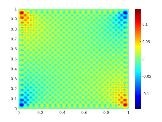
In this example, the permeability coefficient κ\kappa is selected as the piecewise constant function with highly varying. The profile of the permeability inverse is shown in Fig. 1(a). As we know, this example has no analytic solutions.

In Fig. 1, a 128×\times128 rectangular partition is used to solve this example. The profiles of the pressure and the two components of the velocity for CDG are plotted in Fig. 1(b)-1(d)

Refer to caption
(a) Profile of κ1\kappa^{-1}
Refer to caption
(b) Profile of p
Refer to caption
(c) Profile of first component of 𝐮{\mathbf{u}}
Refer to caption
(d) Profile of second component of 𝐮{\mathbf{u}}
Figure 1: Profiles of κ1\kappa^{-1} and numerical solution in Ex. 2

6.3 Example 3

In this example, we choose a vuggy medium with the permeability coefficient κ\kappa highly varying. The profile of the permeability inverse is plotted in Fig. 2(a). For solving this example, a 128×\times128 rectangular partition is used. And the pressure obtained by CDG method is present in Fig. 2(b). The velocity profiles are shown in Fig. 2(c)-2(d).

Refer to caption
(a) Profile of κ1\kappa^{-1}
Refer to caption
(b) Profile of p
Refer to caption
(c) Profile of first component of 𝐮{\mathbf{u}}
Refer to caption
(d) Profile of second component of 𝐮{\mathbf{u}}
Figure 2: Profiles of κ1\kappa^{-1} and numerical solution in EX. 3

6.4 Example 4

The fluid flowing in a fibrous material can also be described by Brinkman equations. Fig. 3(a) shows the inverse of permeability in a common fibrous material. The parameters are the same as in the previous example. We can get the corresponding pressure in Fig. 3(b) and velocity in Fig. 3(c)-3(d) by CDG method.

Refer to caption
(a) Profile of κ1\kappa^{-1}
Refer to caption
(b) Profile of p
Refer to caption
(c) Profile of first component of 𝐮{\mathbf{u}}
Refer to caption
(d) Profile of second component of 𝐮{\mathbf{u}}
Figure 3: Profiles of κ1\kappa^{-1} and numerical solution in EX. 4

Appendix A Some Inequality Estimates

In this Appendix, we provide inequalities for projection operators QhQ_{h}, 𝐐h{\mathbf{Q}}_{h}, h{\mathbb{Q}}_{h} and inequality estimates used in the previous paper.

Lemma A.1.

[22] Let 𝒯h{\mathcal{T}}_{h} be a shape regular partition of Ω\Omega, 𝐰[Hk+1(Ω)]d{\mathbf{w}}\in[H^{k+1}(\Omega)]^{d} and ρHk(Ω)\rho\in H^{k}(\Omega). Then we have the following projection inequalities

T𝒯h𝐰Qh𝐰T2\displaystyle\sum_{T\in\mathcal{T}_{h}}\|{\mathbf{w}}-Q_{h}{\mathbf{w}}\|^{2}_{T} Ch2(k+1)𝐰k+12,\displaystyle\leq Ch^{2(k+1)}\|{\mathbf{w}}\|^{2}_{k+1}, (A.1)
T𝒯h𝐰𝐐h(𝐰)T2\displaystyle\sum_{T\in\mathcal{T}_{h}}\|\nabla{\mathbf{w}}-{\mathbf{Q}}_{h}(\nabla{\mathbf{w}})\|^{2}_{T} Ch2k𝐰k+12,\displaystyle\leq Ch^{2k}\|{\mathbf{w}}\|^{2}_{k+1}, (A.2)
T𝒯hρhρT2\displaystyle\sum_{T\in\mathcal{T}_{h}}\|\rho-{\mathbb{Q}}_{h}\rho\|^{2}_{T} Ch2kρk2.\displaystyle\leq Ch^{2k}\|\rho\|_{k}^{2}. (A.3)

where CC is a constant independent of the size of mesh hh and the functions 𝐰{\mathbf{w}} and ρ\rho.

Let TT be a cell with ee as an edge/face. For any function ρH1(T)\rho\in H^{1}(T), the following trace inequality has been proved to be valid in [22]:

ρe2C(hT1ρT2+hTρT2).\displaystyle\|\rho\|^{2}_{e}\leq C(h^{-1}_{T}\|\rho\|^{2}_{T}+h_{T}\|\nabla\rho\|^{2}_{T}). (A.4)

Furthermore, if ρPk(T)\rho\in P_{k}(T), we have the following inverse inequality

ρTChT1ρT.\displaystyle\|\nabla\rho\|_{T}\leq Ch_{T}^{-1}\|\rho\|_{T}. (A.5)
Lemma A.2.

For any 𝐯Vh{\mathbf{v}}\in V_{h}, the following inequality holds true

ehh1[𝐯]e2C|𝐯|2,\displaystyle\sum_{e\in{\mathcal{E}}_{h}}h^{-1}\|[{\mathbf{v}}]\|^{2}_{e}\leq C|\!|\!|{\mathbf{v}}|\!|\!|^{2}, (A.6)

where CC is a positive constant.

The proof of this lemma is given in Lemma 3.2 in [27].

Lemma A.3.

For any 𝐰[Hk+1(Ω)]d{\mathbf{w}}\in[H^{k+1}(\Omega)]^{d}, rHk(Ω)r\in H^{k}(\Omega) 𝐯Vh{\mathbf{v}}\in V_{h} and qWhq\in W_{h}. Then we have

|l1(𝐰,𝐯)|\displaystyle|l_{1}({\mathbf{w}},{\mathbf{v}})| Chk𝐰k+1|𝐯|,\displaystyle\leq Ch^{k}\|{\mathbf{w}}\|_{k+1}|\!|\!|{\mathbf{v}}|\!|\!|, (A.7)
|l2(𝐰,𝐯)|\displaystyle|l_{2}({\mathbf{w}},{\mathbf{v}})| Chk𝐰k+1|𝐯|,\displaystyle\leq Ch^{k}\|{\mathbf{w}}\|_{k+1}|\!|\!|{\mathbf{v}}|\!|\!|, (A.8)
|l3(r,𝐯)|\displaystyle|l_{3}(r,{\mathbf{v}})| Chkrk|𝐯|,\displaystyle\leq Ch^{k}\|r\|_{k}|\!|\!|{\mathbf{v}}|\!|\!|, (A.9)
|l4(𝐰,q)|\displaystyle|l_{4}({\mathbf{w}},q)| Chk𝐰k+1qh,\displaystyle\leq Ch^{k}\|{\mathbf{w}}\|_{k+1}\|q\|_{h}, (A.10)
|s(hr,q)|\displaystyle|s({\mathbb{Q}}_{h}r,q)| Chkrkqh.\displaystyle\leq Ch^{k}\|r\|_{k}\|q\|_{h}. (A.11)
Proof.

Using the definition of w\nabla_{w}, the Cauchy-Schwarz inequality, the trace inequality (A.4) and the projection inequality (A.1), we obtain

|l1(𝐰,𝐯)|\displaystyle|l_{1}({\mathbf{w}},{\mathbf{v}})| =|T𝒯h(w(𝐰Qh𝐰),w𝐯)T|\displaystyle=\Bigg{|}\sum_{T\in\mathcal{T}_{h}}(\nabla_{w}({\mathbf{w}}-Q_{h}{\mathbf{w}}),\nabla_{w}{\mathbf{v}})_{T}\Bigg{|}
=|T𝒯h((𝐰Qw𝐰,w𝐯)T+{𝐰Qw𝐰},w𝐯𝐧T)|\displaystyle=\Bigg{|}\sum_{T\in\mathcal{T}_{h}}(-({\mathbf{w}}-Q_{w}{\mathbf{w}},\nabla\cdot\nabla_{w}{\mathbf{v}})_{T}+\left<\left\{{\mathbf{w}}-Q_{w}{\mathbf{w}}\right\},\nabla_{w}{\mathbf{v}}\cdot{\mathbf{n}}\right>_{\partial T})\Bigg{|}
=|T𝒯h(((𝐰Qw𝐰),w𝐯)T+Qw𝐰{Qw𝐰},w𝐯𝐧T)|\displaystyle=\Bigg{|}\sum_{T\in\mathcal{T}_{h}}((\nabla({\mathbf{w}}-Q_{w}{\mathbf{w}}),\nabla_{w}{\mathbf{v}})_{T}+\left<Q_{w}{\mathbf{w}}-\left\{Q_{w}{\mathbf{w}}\right\},\nabla_{w}{\mathbf{v}}\cdot{\mathbf{n}}\right>_{\partial T})\Bigg{|}
=|T𝒯h(((𝐰Qw𝐰),w𝐯)T+Qw𝐰𝐰+{𝐰Qw𝐰},w𝐯𝐧T)|\displaystyle=\Bigg{|}\sum_{T\in\mathcal{T}_{h}}((\nabla({\mathbf{w}}-Q_{w}{\mathbf{w}}),\nabla_{w}{\mathbf{v}})_{T}+\left<Q_{w}{\mathbf{w}}-{\mathbf{w}}+\left\{{\mathbf{w}}-Q_{w}{\mathbf{w}}\right\},\nabla_{w}{\mathbf{v}}\cdot{\mathbf{n}}\right>_{\partial T})\Bigg{|}
T𝒯h((𝐰Qw𝐰)Tw𝐯T+Ch12𝐰Qw𝐰Tw𝐯T)\displaystyle\leq\sum_{T\in\mathcal{T}_{h}}(\|\nabla({\mathbf{w}}-Q_{w}{\mathbf{w}})\|_{T}\|\nabla_{w}{\mathbf{v}}\|_{T}+Ch^{-\frac{1}{2}}\|{\mathbf{w}}-Q_{w}{\mathbf{w}}\|_{\partial T}\|\nabla_{w}{\mathbf{v}}\|_{T})
(T𝒯h((𝐰Qw𝐰)T+Ch1𝐰Qw𝐰T)2)12(T𝒯hw𝐯T2)12\displaystyle\leq\left(\sum_{T\in\mathcal{T}_{h}}(\|\nabla({\mathbf{w}}-Q_{w}{\mathbf{w}})\|_{T}+Ch^{-1}\|{\mathbf{w}}-Q_{w}{\mathbf{w}}\|_{T})^{2}\right)^{\frac{1}{2}}\left(\sum_{T\in\mathcal{T}_{h}}\|\nabla_{w}{\mathbf{v}}\|_{T}^{2}\right)^{\frac{1}{2}}
Chk𝐰k+1|𝐯|.\displaystyle\leq Ch^{k}\|{\mathbf{w}}\|_{k+1}|\!|\!|{\mathbf{v}}|\!|\!|.

Combining (A.6), (2.1) and the projection inequality (A.2) gives

|l2(𝐰,𝐯)|\displaystyle|l_{2}({\mathbf{w}},{\mathbf{v}})| =|T𝒯h(𝐰𝐐h𝐰)𝐧,𝐯{𝐯}T|\displaystyle=\Bigg{|}\sum_{T\in\mathcal{T}_{h}}\left<(\nabla{\mathbf{w}}-{\mathbf{Q}}_{h}\nabla{\mathbf{w}})\cdot{\mathbf{n}},{\mathbf{v}}-\left\{{\mathbf{v}}\right\}\right>_{\partial T}\Bigg{|}
C(T𝒯hh𝐰𝐐h𝐰T2)12(ehh1[𝐯]e2)12\displaystyle\leq C\left(\sum_{T\in\mathcal{T}_{h}}h\|\nabla{\mathbf{w}}-{\mathbf{Q}}_{h}\nabla{\mathbf{w}}\|_{\partial T}^{2}\right)^{\frac{1}{2}}\left(\sum_{e\in{\mathcal{E}}_{h}}h^{-1}\|[{\mathbf{v}}]\|_{e}^{2}\right)^{\frac{1}{2}}
Chk𝐰k+1|𝐯|.\displaystyle\leq Ch^{k}\|{\mathbf{w}}\|_{k+1}|\!|\!|{\mathbf{v}}|\!|\!|.

According to the projection inequality (A.3), we get

|l3(r,𝐯)|\displaystyle|l_{3}(r,{\mathbf{v}})| =|T𝒯hrhr,𝐯𝐧T|\displaystyle=\Bigg{|}\sum_{T\in\mathcal{T}_{h}}\left<r-{\mathbb{Q}}_{h}r,{\mathbf{v}}\cdot{\mathbf{n}}\right>_{\partial T}\Bigg{|}
C(T𝒯hhrhrT2)12(ehh1[𝐯]e2)12\displaystyle\leq C\left(\sum_{T\in\mathcal{T}_{h}}h\|r-{\mathbb{Q}}_{h}r\|_{\partial T}^{2}\right)^{\frac{1}{2}}\left(\sum_{e\in{\mathcal{E}}_{h}}h^{-1}\|[{\mathbf{v}}]\|_{e}^{2}\right)^{\frac{1}{2}}
Chkrk|𝐯|.\displaystyle\leq Ch^{k}\|r\|_{k}|\!|\!|{\mathbf{v}}|\!|\!|.

Similarly, with (2.2), then

|l4(𝐰,q)|\displaystyle|l_{4}({\mathbf{w}},q)| =|T𝒯h(𝐮Qh𝐮)𝐧,q{q}T|\displaystyle=\Bigg{|}\sum_{T\in\mathcal{T}_{h}}\left<({\mathbf{u}}-Q_{h}{\mathbf{u}})\cdot{\mathbf{n}},q-\left\{q\right\}\right>_{\partial T}\Bigg{|}
C(T𝒯hh1𝐰Qh𝐰T2)12(eh0h[[q]]e2)12\displaystyle\leq C\left(\sum_{T\in\mathcal{T}_{h}}h^{-1}\|{\mathbf{w}}-Q_{h}{\mathbf{w}}\|_{\partial T}^{2}\right)^{\frac{1}{2}}\left(\sum_{e\in{\mathcal{E}}_{h}^{0}}h\|[\![q]\!]\|_{e}^{2}\right)^{\frac{1}{2}}
Chk𝐰k+1qh.\displaystyle\leq Ch^{k}\|{\mathbf{w}}\|_{k+1}\|q\|_{h}.

Using the definition of s(,)s(\cdot,\cdot), we get

|s(hr,q)|\displaystyle|s({\mathbb{Q}}_{h}r,q)| =|eh0h[[hr]],[[q]]e|\displaystyle=\Bigg{|}\sum_{e\in{\mathcal{E}}_{h}^{0}}h\left<[\![{\mathbb{Q}}_{h}r]\!],[\![q]\!]\right>_{e}\Bigg{|}
=|eh0h[[hrr]],[[q]]e|\displaystyle=\Bigg{|}\sum_{e\in{\mathcal{E}}_{h}^{0}}h\left<[\![{\mathbb{Q}}_{h}r-r]\!],[\![q]\!]\right>_{e}\Bigg{|}
C(T𝒯hhrhrT2)12(eh0h[[q]]e2)12\displaystyle\leq C\left(\sum_{T\in\mathcal{T}_{h}}h\|r-{\mathbb{Q}}_{h}r\|_{\partial T}^{2}\right)^{\frac{1}{2}}\left(\sum_{e\in{\mathcal{E}}_{h}^{0}}h\|[\![q]\!]\|_{e}^{2}\right)^{\frac{1}{2}}
Chkrkqh,\displaystyle\leq Ch^{k}\|r\|_{k}\|q\|_{h},

which completes the proof. ∎

Acknowledgments

This work was supported by National Natural Science Foundation of China (Grant No. 1901015, 12271208), and Key Laboratory of Symbolic Computation and Knowledge Engineering of Ministry of Education, Jilin University. We sincerely thank the anonymous reviewers for their insightful comments, which have helped improve the quality of this paper.

References

  • [1] A. Al-Taweel, and X. Wang, A note on the optimal degree of the weak gradient of the stabilizer free weak Galerkin finite element method, Appl. Numer. Math., 150 (2020), 444-451.
  • [2] V. Anaya, G. N. Gatica, D. Mora and R. Ruiz-Baier, An augmented velocity-vorticity-pressure formulation for the Brinkman equations, Internat. J. Numer. Methods Fluids, 79 (2015), 109-137.
  • [3] A. A. Avramenko, I. V. Shevchuk, M. M. Kovetskaya, and Y. Y. Kovetska, Darcy-Brinkman-forchheimer model for film boiling in porous media, Transp. Porous Media, 134 (2020), 503-536.
  • [4] S. Badia, and R. Codina, Unified stabilized finite element formulations for the Stokes and the Darcy problems, SIAM J. Numer. Anal., 47 (2009), 1971-2000.
  • [5] H. Brinkman, A calculation of the viscous force exerted by a flowing fluid on a dense swarm of particles, Flow Turbul. Combust., 1 (1949), 27-34.
  • [6] E. Cáceres, G. N. Gatica, and F. A. Sequeira, A mixed virtual element method for the Brinkman problem, Math. Models Methods Appl. Sci., 27 (2017), 707-743.
  • [7] B. Cockburn, G. Kanschat and D. Schötzau, A note on discontinuous Galerkin divergence-free solutions of the Navier-Stokes equations, J. Sci. Comput., 31 (2007), 61–73.
  • [8] C. D’Angelo and P. Zunino, A finite element method based on weighted interior penalties for heterogeneous incompressible flows, SIAM J. Numer. Anal., 47 (2009), 3990-4020.
  • [9] L. de Paulo Ferreira, T. D. S. de Oliveira, R. Surmas, M. A. P. da Silva, and R. P. Peçanha, Brinkman equation in reactive flow: Contribution of each term in carbonate acidification simulations, Adv. Water. Resour., 144 (2020), 103696.
  • [10] F. Golfier, D. Lasseux, and M. Quintard, Investigation of the effective permeability of vuggy or fractured porous media from a Darcy-Brinkman approach, Comput. Geosci., 19 (2015), 63-78.
  • [11] J. S. Howell, M. Neilan and N. J. Walkington, A dual-mixed finite element method for the Brinkman problem, SMAI J. Comput. Math., 2 (2016), 1-17.
  • [12] P. Huang and J. Chen, Some low order nonconforming mixed finite elements combined with Raviart-Thomas elements for a coupled Stokes-Darcy model, Jpn. J. Ind. Appl. Math., 30 (2013), 565–584.
  • [13] J. Könnö and R. Stenberg, H(div)-conforming finite elements for the Brinkman problem, Math. Models Methods Appl. Sci. , 21 (2011), 2227-2248.
  • [14] I. Ligaarden, M. Krotkiewski, K. A. Lie, M. Pal and D. W. Schmid, On the Stokes-Brinkman equations for modeling flow in carbonate reservoirs, Oxford: Proceedings of the the ECMOR XII - 12th European Conferenceon the mathematics of Oil Recovery, 2010.
  • [15] K. A. Mardal, X. C. Tai and R. Winther, A Robust Finite Element Method for Darcy - Stokes Flow, SIAM J. Numer. Anal., 40 (2002), 1605-1631.
  • [16] L. Mu, J. Wang, and X. Ye, A stable numerical algorithm for the Brinkman equations by weak Galerkin finite element methods, J. Comput. Phys., 273 (2014), 327-342.
  • [17] Y. Qian, S. Wu, and F. Wang, A mixed discontinuous Galerkin method with symmetric stress for Brinkman problem based on the velocity-pseudostress formulation, Comput. Methods Appl. Mech. Engrg., 368 (2020), 113177.
  • [18] K. Vafai, Porous media: applications in biological systems and biotechnology. Springer Series in Computational Mathematics, 2010, CRC Press, USA.
  • [19] G. Wang, Y. Wang, and Y. He, Two robust virtual element methods for the Brinkman equations, Calcolo, 58 (2021), 49.
  • [20] J. Wang and X. Ye, A weak Galerkin finite element method for second-order elliptic problems, J. Comput. Appl. Math., 241 (2013), 103-115.
  • [21] J. Wang and X. Ye, A weak Galerkin finite element method for the stokes equations, Adv. Comput. Math., 42 (2016), 155–174.
  • [22] J. Wang and X. Ye, A weak Galerkin mixed finite element method for second order elliptic problems, Math. Comp., 83 (2014), 2101-2126.
  • [23] Y. Wang, F. Gao, and J. Cui, A conforming discontinuous Galerkin finite element method for elliptic interface problems, J. Comput. Appl. Math., 412 (2022), 114304.
  • [24] Y. Wang, F. Gao, and J. Cui, A conforming discontinuous Galerkin finite element method for linear elasticity interface problems, J. Sci. Comput., 92 (2022), 20.
  • [25] X. Xie, J. Xu and G. Xue, Uniformly-stable finite element methods for Darcy-Stokes-Brinkman models, J. Comput. Math., 26 (2008), 437-455.
  • [26] X. Ye and S. Zhang, A conforming discontinuous Galerkin finite element method, Int. J. Numer. Anal. Model., 17 (2020), 110-117.
  • [27] X. Ye and S. Zhang, A conforming discontinuous Galerkin finite element method: Part II, Int. J. Numer. Anal. Model., 17 (2020), 281-296.
  • [28] X. Ye and S. Zhang, A conforming discontinuous Galerkin finite element method for the Stokes problem on polytopal meshes, Internat. J. Numer. Methods Fluids, 93 (2021), 1913-1928.
  • [29] Q. Zhai, R. Zhang, and L. Mu, A new weak Galerkin finite element scheme for the Brinkman model, Commun. Comput. Phys., 19 (2016), 1409-1434.
  • [30] X. Zhang and M. Feng, A projection-based stabilized virtual element method for the unsteady incompressible Brinkman equations, Appl. Math. Comp., 408 (2021), 126325.