A Computational Efficient Maximum Likelihood Direct Position Determination Approach for Multiple Emitters Using Angle and Doppler Measurements
Abstract
Emitter localization is widely applied in the military and civilian fields. In this paper, we tackle the problem of position estimation for multiple stationary emitters using Doppler frequency shifts and angles by moving receivers. The computational load for the exhaustive maximum likelihood (ML) direct position determination (DPD) search is insufferable. Based on the Pincus’ theorem and importance sampling (IS) concept, we propose a novel non-iterative ML DPD method. The proposed method transforms the original multi-dimensional grid search into random variables generation with multiple low-dimensional pseudo-probability density functions (PDF), and the circular mean is used for superior position estimation performance. The computational complexity of the proposed method is modest, and the off-grid problem that most existing DPD techniques face is significantly alleviated. Moreover, it can be implemented in parallel separately. Simulation results demonstrate that the proposed ML DPD estimator can achieve better estimation accuracy than state-of-the-art DPD techniques. With a reasonable parameter choice, the estimation performance of the proposed technique is very close to the Cramér-Rao lower bound (CRLB), even in the adverse conditions of low signal-to-noise ratios (SNR) levels.
keywords:
Direct position determination, Maximum likelihood, Importance sampling, Monte-Carlo methods, Circular mean1 Introduction
Localization of the narrowband emitter attracts much interest in radar, sonar, satellite positioning and navigation [1] [2]. Some researchers devoted their attention to the scenario that both emitter and receivers are stationary, the angle of arrival (AOA) of the emitter can be measured by the antenna array in the receiver [3, 4]. The others turned interests to scenarios that moving receivers with stationary emitter [5] and moving receivers with moving emitter [6]. The motion induces a Doppler frequency shift that is proportional to the radial velocity relatively between receiver and emitter. This additional information is the key for estimating location and velocity of the emitter in this case.
In general, two conventional processing steps are involved in traditional localization methods for a single emitter. In the first step, the receiver independently estimates parameters of interest, including direction of arrival (DOA) [7, 8], received signal strength (RSS) [9], time of arrival (TOA) [10] and Doppler frequency shift [11]. In the second step, the location of the emitter is estimated based on the intermediate parameters from the first step. Theoretically, these methods are sub-optimal since the estimation of the parameters in the first step ignores the constraint that all measurements must correspond to the same emitter location and transmitting signal. Furthermore, in the case of multiple emitters, the problem of associating estimated parameters with the corresponding emitter arises.
Different from the conventional two-step approach, a new technology called direct position determination (DPD) estimates the emitter position from received signals straightforwardly [12, 13, 14, 15, 16, 17, 18, 19, 20]. The DPD technology uses the data collected by multiple receivers to formulate a cost function that depends on the location of the emitter. Therefore, it inherently overcomes the parameter-emitter association problem and outperforms two-step methods in low signal-to-noise ratio (SNR) scenarios [12]. Instead of transmitting the intermediate parameters, the DPD technique requires the transmission of received signals to a processing center so that higher communication bandwidth is necessary.
The maximum likelihood (ML) estimator is well known to be an optimal technique for solving the DPD problem. However, for the scenario with multiple stationary emitters and moving receivers, the exact implementation of the ML technique requires a multi-dimensional grid search so that the real-time processing becomes impractical, since the computation resource is usually limited for moving receivers (e.g., unmanned aerial vehicles (UAVs)). To sidestep the exhaustive grid search, many DPD methods have been developed. Assuming the number of observed snapshots are infinite, [13] proposed an approach that approximates the ML problem into multiple low-dimensional optimization problems under the condition that transmitted waveform is known. Yet this method is not applicable for the moving receiver scenario since it is not practical for a receiver to repeat the track and visit the same places with the same velocities several times [16]. A subspace DPD algorithm was proposed in [21] with the assumption that the number of emitters are known. To avoid model order determination, the minimum variance distortionless response (MVDR) concept was considered. [16, 22] proposed a beamforming DPD algorithm based on Doppler frequency shift and AOA, respectively. In practice, the subspace and beamforming approaches are attractive due to the high resolution and modest computational load. However, they are sub-optimal compared to the ML estimator, and suffer from severe performance degradation for low SNR levels, the small number of snapshots and/or closely-spaced emitters, which are common in the moving receiver scenario. On the other hand, many existing ML solutions are iterative with a lower computational cost. The iterative DPD estimator introduced in [15] is based on the alternating projection (AP) technique. [23] proposed a decoupled ML DPD algorithm later, which is also iterative. Nevertheless, the performance of these two ML DPD estimators is closely tied to the initialization, i.e., their ML cost function will not converge to the global maximum if initial guesses deviate significantly from true values. Moreover, the DPD estimators mentioned above select the fixed sampling position grids to serve as a possible set of candidate estimates, based on the assumption that unknown emitter locations are certainly on grids, which leads to the inevitable off-grid problem. Dense grid sampling can alleviate this problem while the cost is an excessive increase in computational complexity. Hence, a non-iterative ML estimator with rapidity needs to be studied, which should also be independent of grid density.
A Monte Carlo technique has been previously proposed for computationally efficient ML estimation of interested parameter[24]. It builds on the global maximization theorem of Pincus [25] and the importance sampling (IS) concept [26]. By choosing an appropriate IS function, the multi-dimensional ML search problem can be factorized into several low-dimensional sub-problems. This method has been applied to the frequency estimation and DOA estimation [27, 28], in which good performance is provided. More recently, it was leveraged in joint angle and Doppler estimation [29], TDOA-based source localization [30], delay estimation and joint angle and delay estimation in multi-path environments [31, 32].
As mentioned before, it is difficult for state-of-the-art DPD techniques to combine computational load and robustness in moving receiver scenarios. Thus resorting to the IS concept is necessary. Some scholars have applied it to the DPD methods [33]. F. Ma [34] exerted IS concept for the distributed DPD, but only one source is considered. Another IS-based DPD approach was proposed in [35] for multiple stationary emitters localization by static receivers using AOA and TOA. In this paper, we apply the IS technique along with the ML concept to the DPD problem for the scenario of moving array receivers and multiple stationary emitters, where the waveform of transmitted signals is known a priori. The study of this paper is not a straightforward extension to [35]. As discussed in Section 4.2, the linear mean should be replaced by circular mean to obtain better position estimation performance in the considered scenario. We reformulate the conventional ML cost function into the form of pseudo-probability density function (PDF). Thus the multi-dimensional maximization is converted to a multi-dimensional integration, which can be well approximated by IS technique and results thereby in tremendous computational savings. Considering the two-dimensional case that emitters are confined to a plane, the multi-dimensional optimization problem can be factorized into several two-dimensional sub-problems, or over a three-dimensional space in the spatial case. Thus the ML estimation of multiple emitter locations boils down to the computation of mean estimate from a number of easily generated realizations, multi-dimensional grid search is avoided. The proposed algorithm considerably alleviates the off-grid problems and can be efficiently executed on multi-processor platforms in an parallel computing implementation.
The contributions of this manuscript are summarized as follows: (1) A computationally efficient non-iterative ML DPD algorithm for multiple emitters is proposed in moving receivers scenario, which transforms the high-dimensional estimation problem into multiple low-dimensional problems. (2) The search process is converted to the generation of samples, thus the off-grid problem is significantly alleviated. (3) The circular mean is applied for the final position estimation rather than the linear mean to enhance accuracy further.
This paper is organized as follows: Section 2 gives the signal model relating to angle and Doppler frequency shift. In Section 3, Pincus’ theorem is applied for the ML estimation of positions of multiple emitters. In Section 4, we derive the importance function and finish position estimation by circular mean, where the main contributions of the paper are given in Sections 4.1 and 4.2. Simulation results are discussed in Section 5. Finally, conclusions are included in Section 6
We define beforehand some of the common notations that will be adopted in this work. Vectors and matrices are represented in lower-case and upper-case bold fonts, respectively. The Euclidean norm of any vector is denoted as , stands for the -dimensional uniform distribution between and . Moreover, , and denote the conjugate, transpose and Hermitian transpose, respectively. stands for the kronecker product and denotes the identity matrix. For a vector , is a diagonal matrix with diagonal elements be , and for a matrix , denotes its -th element. In addition, and return the statistical expectation and complex number’s phase, respectively. Finally, is the pure complex number that verifies , and is used for definitions.
2 Problem formulation
Consider a scenario with moving receivers, each one equipped a uniform linear array (ULA) consisting of elements, the spacing between adjacent elements is . Receivers are assumed to be synchronized in frequency and time.
Assuming that there are stationary radio emitters , is known a priori, the -th emitter location is denoted by a vector of coordinate (for planar geometry and for the spatial case ). All emitters radiate narrowband signals, the waveform and the carrier frequency of signals are known in advance (e.g., the training or synchronization sequences), and the bandwidth of signals is small compared to the inverse of the propagation time over array aperture. Each receiver intercepts the transmitted signals at short intervals along its trajectory. Let vector and (, ) denote the position vector and velocity vector of the -th receiver at the -th interception interval, respectively. Hence, the complex signal vector observed by the -th receiver at the -th interception interval at time is given by
| (1) |
where is the observation time. is an unknown complex attenuation factor that represents the path attenuation from -th emitter to the -th receiver at the -th interception interval. is the transmitting signal from the -th emitter during the -th interception interval, which is a priori knowledge. The noise vector is independent and normally distributed with zero mean and covariance matrix , which can be denoted as . Aussuming that each interception interval is short enough and mutually exclusive, the array vectors and observed frequency are considered quasistatic in each interval. Their expressions are
| (2) |
where denotes the position vector of -th array antenna in the -th receiver at the -th interception interval, and
| (3) |
where
| (4) |
| (5) |
and is the signal’s propagation speed. More details about the observed frequency are given in [14]. As is known to the receiver, after down conversion, the intercepted signal frequency become .
The down converted signal is sampled at where and . For simplicity, , and are represented by , and , respectively. Then the sampled signal can be rewritten in a vector form as
| (6) |
where
| (7) |
3 Formulation of ML estimation
3.1 Concentrated maximum likelihood function
The unknown parameters of interest are given by
| (8) |
where . We focus on the ML estimator that depends on and . Since , the ML estimator coincides with the Least Squares (LS) estimator. Thus the log-likelihood function (after dropping the constant terms) can be given by
| (9) |
where . The path attenuation vectors that maximize (9) are given by
| (10) |
Substituting (10) back into (9) yields the so-called concentrated likelihood function (CLF) which depends solely on
| (11) |
Instead of maximizing (11), we can equivalently maximize
| (12) |
Hence, the ML estimate of is then obtained from the following multi-dimensional optimization problem
| (13) |
3.2 Global maximization of the CLF
A direct solution of (13) requires -dimensional search, which is extremely computational challenging. To solve this problem, we resort to the Pincus’ theorem [25]. It provides a mean for performing the nonlinear multi-dimensional optimization and guarantees to produce the global maximum. The Pincus’ theorem states that the vector yields the unique global maximum of a continuous -dimensional function , whose -th entry is given by
| (14) |
Using a sufficiently large to replace , the limit in (14) is approximated as
| (15) |
Applying (15) to the optimization problem (13) with and , and letting for simplifying the exhibition, the expressions for the estimation of the are given by
| (16a) | ||||
| (16b) | ||||
where and denote x-coordinate and y-coordinate of the -th emitter, respectively. is the normalized function of defined as
| (17) |
However, it is difficult to directly deal with the multi-dimensional integral (16a) and (16b). Closely inspecting (17), satisfies . Considering as a pseudo-PDF of , thus the estimation of in (16a) and (16b) can be alternatively regarded as statistical expectations
| (18) |
Intuitively, we can approximate the expectations in (18) with the generation of realizations distributed according to ,
| (19) |
In this way, the complicated integrations can be approximated by the sample mean estimates. Clearly, according to the law of large numbers [36], the sample mean estimate will converge to the corresponding expectation as . Thus the increase of results in the decrease of the variance of and . Unfortunately, is still highly non-linear and cannot be practically used to generate . We shall resort to the IS concept and approximately find a simple PDF for realization generation.
4 Position estimation using importance sampling
4.1 Utilization of the importance sampling function
Equations (16a) and (16b) are equivalent to the following forms respectively
| (20a) | ||||
| (20b) | ||||
where is the other pseudo-PDF called importance function [27] [37]. is generally designed as a simple function of for easily generating realizations , which is also desired as similar as possible to . Thus (20a) and (20b) are regarded as computing expectation of transformed random variables
| (21) |
where
| (22) |
Now we turn into the approximate choice for . In order to generate easily, intuitively shall be designed separable in terms of the emitter locations
| (23) |
where is a pseudo-PDF of . in form (23) can be regarded as a joint pseudo-PDF corresponding to multiple mutually independent random variables, which can be easily generated using . Hence, considering the design of shall be appropriate approximation of satisfies (23).
Revisiting (12), can be approximated as a separable function under the condition that is replaced by an invertible diagonal matrix. It can be observed that the entry in the -th row and the -th column of matrix can be expressed as
| (24) |
The diagonal elements are
| (25) |
We verify statistically that the off-diagonal entries of are much smaller compared to with a high probability for almost all possible emitter loactions. To this end, let us define
| (26) |
as the ratio of the off-diagonal entries over diagonal entries of . Then, a large number of random variable vectors and are generated, which are independent identically distributed (IID) in Km, to compute the complementary cumulative distribution function (CCDF) of .
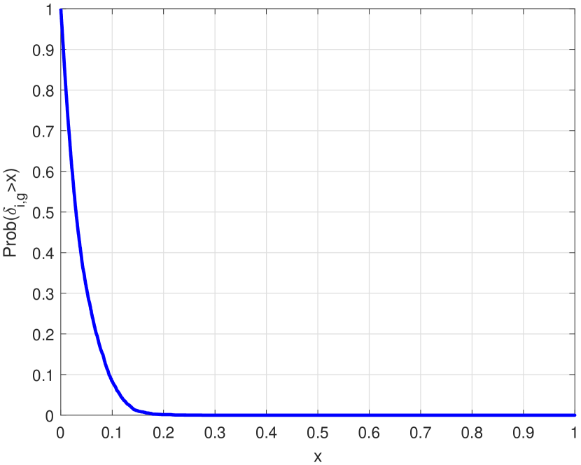
As shown in Fig.1, is indeed dominant compared to corresponding off-diagonal elements, since almost has a zero probability to exceed 0.15. Therefore, a valid approximation for (24) can be obtained
| (27) |
Substituting (27) into (12), is approximately in proportion to the superposition of separated terms
| (28) |
where
| (29) |
Then, the importance function (23) is transformed to
| (30) |
where is the new design parameter involving factor . It should be noted that the choices of and affect the performance of the proposed estimator. can indeed be factorized in terms of the emitter locations as (23), where is expressed as
| (31) |
Thus the generation of can be approximated as generating with bivariate distribution (31), which can be implemented separately and run in parallel with a much faster and less complex execution.
One specific way for generating required vector realizations is based on the inverse probability transformation applied in [36]. Let be the cumulative distribution function (CDF) of random variable vector and generating IID uniform random numbers, i.e., . Thus the variable vector realization can be generated as
| (32) |
However, this way still requires a two-dimensional search process for generating . Recalling (31) that depicts a joint distribution, thus can be factorized as the product of a marginal PDF and a conditional PDF as follows
| (33a) | ||||
| (33b) | ||||
where is the marginal PDF of x-coordinate and is the conditional PDF of y-coordinate given . The definition of and is in the same manner. can be given by
| (34) |
which is used to generate the realization . Then the conditional PDF of given can be expressed as following
| (35) |
By (35) the realization is generated, thus the two-dimensional search process for generating is converted to two line search. We have just showed the process for generating firstly and then . The generation of using and then with is straightforward.
4.2 Emitter location estimation
Recalling the expression of and in (21) and using the IS function defined in (30), the position estimator of the -th emitter can be equivalent to estimate the linear mean [35] of generated realizations
| (36) |
where
| (37) |
However, the linear mean just averages all realizations without considering the existence of outlier seeds, which may result in the inevitable estimation bias. An improvement is using the circular mean [38] instead. As mentioned in [32], under the condition that is as high as desired, the circular mean estimation corresponds to the realization that minimizes the Euclidean distance to the true parameter. For a given random variable , let be a transformation of , then the circular mean of can be expressed as
| (38) |
where are the realizations of random variable .
Assuming that the x-coordinates and y-coordinates of all emitters are in the range and , respectively. Then the alternative formulation of the estimators shown in (21) using circular mean are expressed as
| (39a) | ||||
| (39b) | ||||
where
Note the normalization integral term in will not affect the result of in (39a) and (39b), which can be omitted to reduce the computational load. Actually, defining the weighting coefficient as
| (40) |
and replacing with in (39a) and (39b) can further reduce the computational consumption and guarantee the accuracy [28].
4.3 Implementation details
For the sake of clarity, we give all the necessary details for the location estimation of all emitters by importance sampling as follows:
-
STEP 1:
Derive separable term by (29) for every with the complex signal vectors observed from all interception intervals.
-
STEP 2:
Choose grid points in coordinate range . All grid points have discretization steps and (). Then, by approximating integrals with discrete sums, the pseudo-PDF for every can be approximated as
(41) - STEP 3:
-
STEP 4:
Generate uniform random numbers and perform linear interpolation to for the generation of position x-coordinate realizations
(44) -
STEP 5:
Compute the the conditional PDF of given with linear interpolation
(45) -
STEP 6:
Evaluate the CDF as similarly as (43) and generate uniform random numbers .
-
STEP 7:
Similarly as (44), obtain position y-coordinate realizations with , using linear interpolation technique as well.
- STEP 8:
-
STEP 9:
Finally estimate the location for the -th emitter
| (46a) | ||||
| (46b) | ||||
Note that with linear interpolation technique, the position realizations are not confined to be on grid points. Hence, the proposed IS-DPD does not suffer from the serious off-grid problem.
4.4 Complexity analysis
This part evaluates the complexity of the proposed IS-based estimator. The complexity is counted through the order of the number of complex-valued multiply operations. Most of the computational resource is consumed by obtaining the discretized importance function, generating realizations and evaluating the weighting coefficient. According to the definition of , for one emitter the complexity for obtaining the discretized importance function is . As there are Q emitters, each emitter have realization pairs, recalling STEP 3-STEP 7, the complexity of realization generation is . (40) involves the matrix inverse, whose computational complexity is . So the total computational complexity of the IS-DPD is . On the other hand, the computational complexity of the exhaustive ML grid search algorithm is , it can be seen that when , which is commmon in the moving receiver scenario, the new IS-based ML DPD estimator exhibits remarkable computational savings. These observation are summarized in Table 1. The relative processing time (Rel. Proc. Time) with respect to the proposed method is obtained in a scenario with moving receivers as Fig. 2, where and .
| Algorithm | Complexity | Rel. Proc. Time |
|---|---|---|
| IS-DPD | 1 | |
| Exhaustive ML search | 9091 |
5 Simulation results
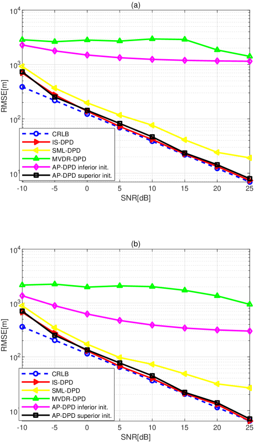
To evaluate the performance of the proposed IS-based DPD approach, we compare it with the AP-DPD algorithm [15] that is one of the iterative implementations of ML-type methods, the SML-DPD and MVDR-DPD proposed in [16], which are beamforming-based methods. The position estimation performance is evaluated in terms of the root mean square error (RMSE)
| (47) |
where is the number of ensemble runs for each test point. is the estimated -th emitter position at the -th trial. The proposed method and aforementioned algorithms are compared with the Camér-Rao lower bound (CRLB) [17], which reflects the theoretical achievable performance taken as a benchmark for all considered algorithms.
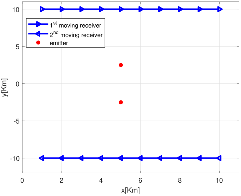
Consider two moving receivers equipped with ULA consisting of half-wavelength spaced elements. They move from Km to Km and Km to Km, respectively. The receivers intercept emitted signals from interested emitters once moving 1 Km each, thus in this case. The scenario is depicted as Fig. 2. The length of the observation time interval is ms and the receivers’ speed is 300 m/s. The orientation of the array is the same as the moving direction of the corresponding receiver. Emitters are located in a square area of Km Km, transmitting flat narrowband Gaussian signals with equal power and bandwidth KHz, the number of emitters is a priori knowledge. The signal carrier frequency is GHz, and the signal propagation speed is set as m/s. The waveform of transmitted signals is known. The down-converted signal is sampled at 10 KHz (by complex sampling) in each interception interval, i.e., each test uses samples. For each emitter, the channel attenuation is randomly generated following the normal distribution with mean one and standard deviation 0.1, and the channel phase is selected from uniformly. The ensemble runs is .
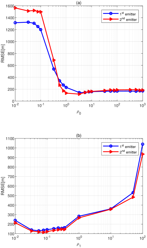
As mentioned in Section 4.1, and are design parameters that should be carefully chosen. To investigate the effect of each parameter on the estimation performance, we vary one of them and fix another one. The scenario contains two emitters located at Km and Km . The rest parameters are fixed at , Km and Km. Fig. 3 shows the performance of the IS-based DPD estimator at SNR=25 dB versus (vs.) and . When the value of is small, the estimator exhibits very poor estimation performance as seen in Fig. 3a. Increasing can remarkably improve the estimation accuracy. This is reasonable because it can be easily inferred from the infinite limit involved in Pincus’ theorem. On the other hand, as illustrated in Fig. 3b, the optimal value of is between 0.005 and 0.1, since this design parameter is used to control the spans of the main lobes of and . Small may not neutralize the effect of the additive noise, while a too large value renders the main lobes be extremely narrow, leading to the true position always lies outside. Large estimation bias is inevitable in both aforementioned conditions. In the following simulations, and are set as 100 and 0.035, respectively.
The next experiment evaluates the impact of the parameter on the performance of the proposed DPD estimator at SNR=5 dB. Other parameters remain the same as above. The results in Fig. 4 match well with the well-known estimation theory that a large enough value of contributes to the consistent mean estimation for (46a) and (46b). However, the computational load inevitably increases as becomes larger. Using a relatively small value such as yields a satisfactory trade-off between performance and complexity, since the accuracy increases insignificantly when is larger than 1000. In the following simulations, is fixed at 1000.
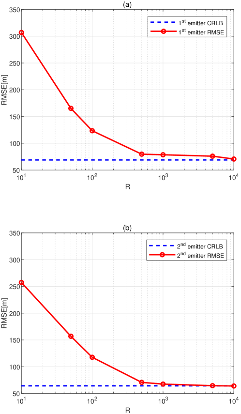
Fig. 5 presents the RMSE of position estimation for varying SNR. The MVDR-DPD estimator passes the received signals through digital Chebyshev type I filters and uses the resulted outputs as snapshots. The peak-to-peak ripple of the set of filters is 0.5 dB. The order of the first and the last filters is 3, while the rest are of order 6. The passband of the -th filter (normalized by bandwidth ) is given by
| (48) |
And for the AP-DPD algorithm, we consider two cases that the initial position of the iterative process is far from and close to the true emitter position. Fig. 5 shows the estimation accuracy of the proposed IS-based DPD estimator is very close to the CRLB. The AP-DPD with a good initialization can achieve similar performance as IS-DPD. However, when the initial guess is far away from the true value, the performance of AP-DPD deteriorates significantly. The MVDR-DPD fails in resolving emitters thus it performs poorly. SML-DPD is inferior to IS-DPD because the correlation among emitters is neglected. The simulation results validate that the IS-DPD is a more robust and accurate implementation of the ML estimator.
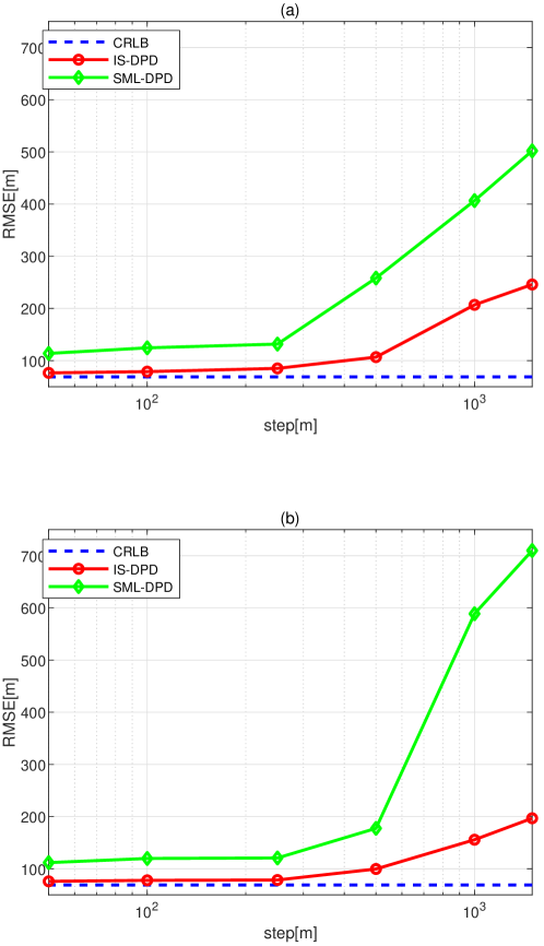
So far, comparisons have been performed versus SNR. To study the influence of the grid density on the performance of different estimators, we vary the grid step with SNR fixed at 5 dB, the true locations of two emitters are unchanged. The SML-DPD is compared as one representative example of the grid-based algorithm. It can be seen from Fig. 6 that, as the grid step gets larger, the estimate becomes less accurate for all methods. Nevertheless, the estimation performance of IS-DPD is still superior to that of SML-DPD. Apparently different from the proposed IS-based estimator, SML-DPD is restricted by the grid step. The results in Fig. 6 match well with the theoretical results in Section 1 and Section 4.3, which shows the benefit due to the utilization of linear interpolation in proposed DPD estimator. Advancing the other DPD methods, the off-grid problem in IS-DPD can be considerably mitigated.
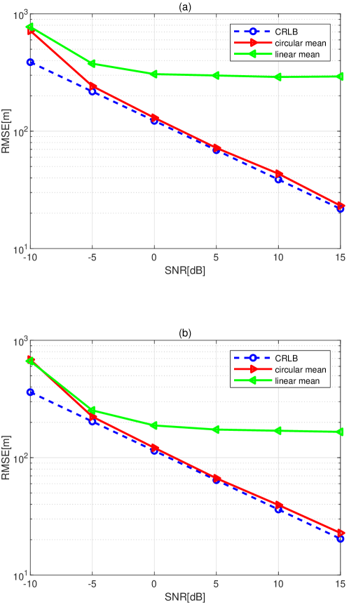
In the last experiment, we focus on the impact of the way for estimating sample mean in the proposed IS-DPD algorithm. Fig. 7 shows the RMSE of position estimation with linear mean and circular mean vs. SNR. Applying the linear mean of samples in the IS-DPD results in a large estimation bias, thus it can be observed that the performance deviates from the CRLB, and the gap between the RMSE and CRLB becomes larger as the SNR increases. The substitution of the linear mean by circular mean significantly reduces the estimation bias and contributes to RMSE achieving the CRLB level. The simulation results validate the advantage of the proposed circular mean based IS-DPD algorithm.
6 Conclusion
This paper discusses location estimation of multiple stationary narrowband radio-frequency emitters based on angle and Doppler shift measurements, where the transmitted signals are observed by multiple moving array receivers. We developed a new implementation of DPD ML estimation, as the number of emitters and the transmitted signal waveform are known a priori. Based on the importance sampling concept, the computational complexity of the new ML DPD algorithm is significantly lower than the traditional multi-dimensional grid search methods, and the off-grid problem is alleviated. Moreover, the proposed method can be implemented separately and run in parallel. In addition, it does not require initial parameter estimates but still guarantees global optimality of the likelihood function. Simulation results show the superiority of the proposed IS-DPD over the state-of-the-art DPD methods in both accuracy and robustness.
Acknowledgments
This work was supported in part by the National Natural Science Foundation of China (NSFC) under Grant 61771108.
References
- [1] D. J. Torrieri, Statistical theory of passive location systems, IEEE Trans. Aerosp. Electron. Syst. (2) (1984) 183–198.
- [2] L. Yang, K. Ho, An approximately efficient TDOA localization algorithm in closed-form for locating multiple disjoint sources with erroneous sensor positions, IEEE Trans. Signal Process. 57 (12) (2009) 4598–4615.
- [3] Y. Sun, K. Ho, Q. Wan, Eigenspace solution for AOA localization in modified polar representation, IEEE Trans. Signal Process. 68 (2020) 2256–2271.
- [4] F. Zhang, Y. Sun, Q. Wan, Calibrating the error from sensor position uncertainty in TDOA-AOA localization, Signal Process. 166 (2020) 107213.
- [5] A. J. Weiss, Direct geolocation of wideband emitters based on delay and Doppler, IEEE Trans. Signal Process. 59 (6) (2011) 2513–2521.
- [6] K. Ho, X. Lu, L.-o. Kovavisaruch, Source localization using TDOA and FDOA measurements in the presence of receiver location errors: Analysis and solution, IEEE Trans. Signal Process. 55 (2) (2007) 684–696.
- [7] J.-D. Lin, W.-H. Fang, Y.-Y. Wang, J.-T. Chen, FSF MUSIC for joint DOA and frequency estimation and its performance analysis, IEEE Trans. Signal Process. 54 (12) (2006) 4529–4542.
- [8] Z. Wang, S. A. Zekavat, A novel semidistributed localization via multinode TOA–DOA fusion, IEEE Trans. Veh. Technol. 58 (7) (2009) 3426–3435.
- [9] S. Tomic, M. Beko, R. Dinis, RSS-based localization in wireless sensor networks using convex relaxation: Noncooperative and cooperative schemes, IEEE Trans. Veh. Technol. 64 (5) (2014) 2037–2050.
- [10] N. Patwari, A. O. Hero, M. Perkins, N. S. Correal, R. J. O’dea, Relative location estimation in wireless sensor networks, IEEE Trans. Signal Process. 51 (8) (2003) 2137–2148.
- [11] A. Tahat, G. Kaddoum, S. Yousefi, S. Valaee, F. Gagnon, A look at the recent wireless positioning techniques with a focus on algorithms for moving receivers, IEEE Access 4 (2016) 6652–6680.
- [12] A. J. Weiss, Direct position determination of narrowband radio transmitters, in: Proc. IEEE Int. Conf. Acoust., Speech, Signal Process., Vol. 2, 2004, pp. ii–249.
- [13] A. J. Weiss, A. Amar, Direct position determination of multiple radio signals, EURASIP J. Adv. Signal Process. 2005 (1) (2005) 1–13.
- [14] A. Amar, A. J. Weiss, Localization of narrowband radio emitters based on Doppler frequency shifts, IEEE Trans. Signal Process. 56 (11) (2008) 5500–5508.
- [15] M. Oispuu, U. Nickel, Direct detection and position determination of multiple sources with intermittent emission, Signal Process. 90 (12) (2010) 3056–3064.
- [16] T. Tirer, A. J. Weiss, High resolution localization of narrowband radio emitters based on Doppler frequency shifts, Signal Process. 141 (2017) 288–298.
- [17] T. Qin, Z. Lu, B. Ba, D. Wang, A decoupled direct positioning algorithm for strictly noncircular sources based on Doppler shifts and angle of arrival, IEEE Access 6 (2018) 34449–34461.
- [18] F. Ma, Z.-M. Liu, F. Guo, Direct position determination for wideband sources using fast approximation, IEEE Trans. Veh. Technol. 68 (8) (2019) 8216–8221.
- [19] H. Zhao, N. Zhang, Y. Shen, Beamspace direct localization for large-scale antenna array systems, IEEE Trans. Signal Process. 68 (2020) 3529–3544.
- [20] K. Hao, Q. Wan, Sparse bayesian inference-based direct off-grid position determination in multipath environments, IEEE Wirel. Commun. Lett. 10 (6) (2021) 1148–1152.
- [21] B. Demissie, M. Oispuu, E. Ruthotto, Localization of multiple sources with a moving array using subspace data fusion, in: Proc. IEEE 11th Int. Conf. Inf. Fusion, 2008, pp. 1–7.
- [22] K. Hao, Q. Wan, High resolution direct detection and position determination of sources with intermittent emission, IEEE Access 7 (2019) 43428–43437.
- [23] T. Qin, L. Li, Z. Lu, D. Wang, A ML-based direct localization method for multiple sources with moving arrays, in: Proc. IEEE 18th Int. Conf. Commun. Technol., 2018, pp. 1073–1076.
- [24] S. Saha, S. M. Kay, Maximum likelihood parameter estimation of superimposed chirps using Monte Carlo importance sampling, IEEE Trans. Signal Process. 50 (2) (2002) 224–230.
- [25] M. Pincus, Letter to the editor—A closed form solution of certain programming problems, Oper. Res. 16 (3) (1968) 690–694.
- [26] R. Y. Rubinstein, D. P. Kroese, Simulation and the Monte Carlo method, Vol. 10, John Wiley & Sons, 2016.
- [27] S. Kay, S. Saha, Mean likelihood frequency estimation, IEEE Trans. Signal Process. 48 (7) (2000) 1937–1946.
- [28] H. Wang, S. Kay, S. Saha, An importance sampling maximum likelihood direction of arrival estimator, IEEE Trans. Signal Process. 56 (10) (2008) 5082–5092.
- [29] H. Wang, S. Kay, Maximum likelihood angle-Doppler estimator using importance sampling, IEEE Trans. Aerosp. Electron. Syst. 46 (2) (2010) 610–622.
- [30] G. Wang, H. Chen, An importance sampling method for TDOA-based source localization, IEEE Trans. Wireless Commun. 10 (5) (2011) 1560–1568.
- [31] A. Masmoudi, F. Bellili, S. Affes, A. Stéphenne, A maximum likelihood time delay estimator in a multipath environment using importance sampling, IEEE Trans. Signal Process. 61 (1) (2012) 182–193.
- [32] F. Bellili, S. B. Amor, S. Affes, A. Ghrayeb, Maximum likelihood joint angle and delay estimation from multipath and multicarrier transmissions with application to indoor localization over IEEE 802.11ac radio, IEEE Trans. Mobile Comput. 18 (5) (2019) 1116–1132.
- [33] F. Ma, F. Guo, L. Yang, Direct position determination of moving sources based on delay and Doppler, IEEE Sensors J. 20 (14) (2020) 7859–7869.
- [34] F. Ma, Z.-M. Liu, F. Guo, Distributed direct position determination, IEEE Trans. Veh. Technol. 69 (11) (2020) 14007–14012.
- [35] K. Hao, Q. Wan, Importance sampling based direct maximum likelihood position determination of multiple emitters using finite measurements, Signal Process. 186 (2021) 108111.
- [36] S. Kay, Intuitive probability and random processes using MATLAB®, Springer Science & Business Media, 2006.
- [37] A. Doucet, N. De Freitas, N. J. Gordon, et al., Sequential Monte Carlo methods in practice, Vol. 1, Springer, 2001.
- [38] K. V. Mardia, Statistics of directional data, Academic press, 2014.