A Chirplet Transform-based Mode Retrieval Method for Multicomponent Signals with Crossover Instantaneous Frequencies
Abstract
In nature and engineering world, the acquired signals are usually affected by multiple complicated factors and appear as multicomponent nonstationary modes. In such and many other situations, it is necessary to separate these signals into a finite number of monocomponents to represent the intrinsic modes and underlying dynamics implicated in the source signals. In this paper, we consider the mode retrieval of a multicomponent signal which has crossing instantaneous frequencies (IFs), meaning that some of the components of the signal overlap in the time-frequency domain. We use the chirplet transform (CT) to represent a multicomponent signal in the three-dimensional space of time, frequency and chirp rate and introduce a CT-based signal separation scheme (CT3S) to retrieve modes. In addition, we analyze the error bounds for IF estimation and component recovery with this scheme. We also propose a matched-filter along certain specific time-frequency lines with respect to the chirp rate to make nonstationary signals be further separated and more concentrated in the three-dimensional space of CT. Furthermore, based on the approximation of source signals with linear chirps at any local time, we propose an innovative signal reconstruction algorithm, called the group filter-matched CT3S (GFCT3S), which also takes a group of components into consideration simultaneously. GFCT3S is suitable for signals with crossing IFs. It also decreases component recovery errors when the IFs curves of different components are not crossover, but fast-varying and close to one and other. Numerical experiments on synthetic and real signals show our method is more accurate and consistent in signal separation than the empirical mode decomposition, synchrosqueezing transform, and other approaches.
(Note: This is the revised paper of “A separation method for multicomponent non-stationary signals with crossover instantaneous frequencies,” which was submitted to IEEE Trans IT on Feb 14, 2020, ms # IT-20-0113. Compared to the original paper, some references were added. In addition, mode retrieval comparison results with Fast-IF and ACMD were provided.)
Keywords: chirplet transform, filter-matched chirplet transform, signal separation, mode retrieval, multicomponent signals with crossing instantaneous frequencies.
1 Introduction
This paper studies blind source nonstationary signal separation in which a nonstationary signal is represented as a superposition of Fourier-like oscillatory modes:
| (1) |
with and varying slowly. Such a representation, called an adaptive harmonic model (AHM) representation, is important for extracting information, such as the underlying dynamics, hidden in the nonstationary signal, with the trend , instantaneous amplitudes (IAs) and the instantaneous frequencies (IFs) being used to describe the underlying dynamics.
In nature, many real-world phenomena that can be formulated as signals (or in terms of time series) are often affected by a number of factors and appear as time-overlapping multicomponent signals in the form of (1). A natural approach to understand and process such phenomena is to decompose, or even better, to separate the multicomponent signals into their basic building blocks (called components, modes or sub-signals) for extracting the necessary features. Also, for radar, communications, and other applications, signals often appear in multicomponent modes. Since these signals are mainly nonstationary, meaning the amplitudes and/or phases of some or all components change with the time, there have been few effective rigorous methods available for decomposition of them.
The empirical mode decomposition (EMD) algorithm along with the Hilbert spectrum analysis (HSA) is a popular method to decompose and analyze nonstationary signals [1]. EMD works like a filter bank [2, 3] to decompose a nonstationary signal into a superposition of intrinsic mode functions (IMFs) and a trend, and then the IF of each IMF is calculated by HSA. There are many articles studying the properties of EMD and variants of EMD have been proposed to improve the performance, see e.g. [2]-[14]. In particular, the separation ability of EMD was discussed in [4], which shows that EMD cannot decompose two components when their frequencies are close to each other. The ensemble EMD (EEMD) was proposed to suppress noise interferences [5]. The original EMD was extended to multivariate signals in [6, 8, 3]. Alternative sifting algorithms and formulations for EMD were introduced in [7, 9, 11]. Similar to the EMD filter bank, the wavelet filter bank for signal decomposition was proposed in [12], called empirical wavelet transform. An EMD-like sifting process was recently proposed in [13] to extract signal components in the linear time-frequency (TF) plane one by one. EMD is an efficient data-driven approach and no basis of functions is required. A weakness of EMD or EEMD is that it can easily lead to mode mixtures or artifacts, namely undesirable or false components [15]. In addition, there is no mathematical theorem to guarantee the recovery of the components.
Time-frequency analysis is another method to separate multicomponent signals, which is widely used in engineering fields such as communication, radar and sonar as a powerful tool for analyzing signals [16]. Time-frequency signal analysis and synthesis using the eigenvalue decomposition method have been studied [17, 18, 19]. Recently the synchrosqueezing transform (SST) was developed in [20] to provide mathematical theorems to guarantee the component recovery of nonstationary multicomponent signals. The SST, which was first introduced in 1996, intended for speech signal separation [21], is based on the continuous wavelet transform (CWT). The short-time Fourier transform (STFT)-based SST was also proposed in [22, 23] and further studied in [24]. SST provides an alternative to the EMD method and its variants, and it overcomes some limitations of the EMD and EEMD schemes [25, 26]. SST has been used in machine fault diagnosis [27, 28], crystal image analysis [29, 30], welding crack acoustic emission signal analysis [31], medical data analysis [32, 33, 34], etc.
SST works well for sinusoidal signals, but not for broadband time-varying frequency signals. To provide sharp representations for signals with significantly frequency changes, two methods were proposed. One is the matching demodulation transform-based SST (or called the instantaneous frequency-embedded SST) proposed in [35, 36] which changes broadband signals to narrow-band signals (see also [37]). The instantaneous frequency-embedded SST proposed in [36] preserves the IFs of the original signals. The other method is the 2nd-order SST introduced in [38] and [39]. The higher-order FSST was presented in [40] and [41], which aims to handle signals containing more general types. Very recently an adaptive SST with a time-varying parameter were introduced in [42, 43]. They obtained the well-separated condition for multicomponent signals using the linear frequency modulation to approximate a nonstationary signal at any local time. In addition, theoretical analysis of adaptive SST was obtained in [44, 45]. SST with a time-varying window width has also been studied in [46, 47].
Recently, a direct time-frequency approach, called signal separation operator (SSO), was introduced in [48] for multicomponent signal separation. In SSO approach, the components are reconstructed simply by substituting the time-frequency ridge to SSO. SSO based on CWT was proposed in [49, 50]. More recently, [51] proposed SSO of “linear chirp-based model” with the phase functions of the signal components in the source signal model (1) approximated by quadratic polynomials at any local time. This model provides a more accurate component recovery formulae, with analysis established in [52, 50].
While SST and SSO are mathematically rigorous on IF estimation and component recovery, both of them require that the components are well-separated in the time-frequency plane, namely IFs of satisfy
| (2) |
for some . In many applications, multicomponent signals are overlapping in the time-frequency plane, that is the IFs of its components are crossover. For example, in radar signal processing, the micro-Doppler

|

|
effects are represented by highly nonstationary signals, when the target or any structure on the target undergoes micro-motion dynamics, such as mechanical vibrations, rotations, or tumbling and coning motions [53, 54]. Figure 1 shows simulated micro-Doppler modulations (two sinusoidal signals) induced by two target’s tumbling motions and their short-time Fourier transforms (SFTFs). In practice we need to recover each components or at least the main body signature corresponding to the target’s motion in the radar signal processing.
We say two components and in (1) are overlapping in time-frequency plane when the IF curves of them are crossing at , i.e., . In this paper we consider multicomponent signals of the form (1) satisfying
| (3) |
where is the regularization parameter and is called the separation resolution. When , (3) is reduced to the well-separated condition (2) required for SST and SSO. Condition (3) allows the IFs of some components to cross as long as their chirp rates are different near the time where IFs crossing occurs.
Recently, many studies have been devoted to estimations of crossing instantaneous frequencies. An algorithm based on linear least square fitting technique was introduced [55]. In [56], the authors employed a three-dimensional parameter space (time, frequency, chirp rate) to estimate instantaneous frequencies and chirp rates jointly of signal, which can make the crossing of IFs appear as separated in the time-frequency-chirprate domain. Furthermore, [56] proposed a three-dimensional ridge detection algorithm. [57] used time-frequency analysis and Radon transform for the unsupervised separation of frequency modulated signals in noisy environment. The chirp rates were also introduced in [58], where estimations of IFs were turned into the resolution of a two-dimensional linear system. Effective quasi maximum likelihood–random samples consensus algorithm was also proposed for IF estimation of overlapping signals in the time-frequency (TF) plane [59].
Moreover, [54] developed a compressive sensing approach to recover stationary narrowband signals contaminated by strong nonstationary signals. An algorithm for estimations of IFs of signals with intersecting signatures in the time-frequency domain is proposed in [60]. Using the estimated IF, the corresponding component is removed from the mixture signal based on de-chirping method [60]. [61] combined parameterized de-chirping and band-pass filter to obtain components of multi-component signal, which avoided dealing with time-frequency representation of the signal and worked well under heavy noise. [62] introduced a novel nonparametric algorithm called ridge path regrouping to extract the IFs of the overlapped components and recover the corresponding component by using the intrinsic chirp component decomposition method. The time-frequency distribution (with a cross-term) [63] was used to estimate IFs. In [64], the authors developed a general model to characterize multi-component chirp signals, where IFs and instantaneous amplitudes of the intrinsic chirp components were modeled as Fourier series. Similarly, a multivariate intrinsic chirp mode was defined in [65]. Then IFs can be estimated using the framework of the general parameterized time-frequency transform and the corresponding multivariate intrinsic chirp modes were reconstructed by solving multivariate linear equations through an extended least square method [65]. Variational nonlinear chirp mode decomposition was employed to separate close or even crossed modes in [66]. In [67], the blind source was decomposed into a series of nonlinear chirp components and the reconstructed nonlinear chirp components can be clustered into corresponding intrinsic chirp sources. The frequency-domain intrinsic component decomposition method was proposed to characterize nonlinear and non-monotonic nonlinear group delays in frequency domain by using different kernel functions and separate and reconstruct each mode simultaneously as a time-frequency filter [68]. An adaptive chirp mode pursuit was proposed to capture signal modes one by one in a recursive framework [69]. In [70], the authors transformed a two-dimensional sinusoidal pattern into a single point in a two-dimensional plane and reconstructed signals from a reduced set of observations (back-projections).
In this paper, using the idea of SSO, we propose a chirplet transform-based signal separation scheme (CT3S) to retrieve modes of multicomponent signals with crossover IFs. Our algorithm addresses the inverse transform and aims to retrieve modes of multicomponent signals with fast varying IFs, even crossing IFs, while the aforementioned papers use the chirplet transform to obtain IFs. Most importantly, we provide a mathematically rigorous theorem which guarantees the recovery of components of multicomponent signals satisfying (3) with CT3S. To our best knowledge, there is no existing literature that establishes mathematical theorems to guarantee the recovery of the components overlapping in the time-frequency plane. Furthermore, we use a matched-filter along the specific time-frequency lines respect to the chirp rate to make different components be further separated and more concentrated in the three dimensional space of the chirplet transform. Based on the approximation of source signals with linear chirps at any local time, we propose an innovative signal reconstruction algorithm, called group filter-matched CT3S (GFCT3S), which takes a group of components into consideration simultaneously. GFCT3S is more suitable for signals with crossing IFs. When the IFs curves of different components are not crossover, but fast-varying and close to each other, our reconstruction algorithm will decrease the recovery errors significantly.
The remainder of this paper is organized as follows. In Section 2, we first review the signal separation methods by SST and SSO. After that we state the problem of recovering sub-signals with crossing IFs. In Section 3, we state our theorem which guarantees the recovery of components for multicomponent signal satisfying (3) with CT3S. We also introduce the filtered chirplet transform and propose GFCT3S for separating multicomponent signals with fast-varying and crossing IFs. We present the numerical experiments in Section 4. A conclusion is then presented in Section 5.
2 Problem statement
The (modified) STFT of signal with a window function is defined by,
| (4) |
If , then the original signal can be recovered back from its STFT:
| (5) |
For multicomponent signal in (1) satisfying the separation condition (2), the sub-signal can be recovered by
| (6) |
for some .
To enhance the time-frequency resolution and concentration, the idea of SST is to reassign the frequency variable. As in [22], denote
| (7) |
The quantity is called the “phase transformation” [20]. The STFT-based SST is to reassign the frequency variable by transforming the STFT of to a quantity, denoted by , on the time-frequency plane:
| (8) |

|
|
||

|

|

|

|

|

|

|

|

|

|

|

|
One also has a reconstruction formula of similar to (6) with replaced by .
Observe that signal reconstructions with the STFT and SST depend on the IF estimation of and a given threshold , hence it is indirect. In contrast, signal separation operator (SSO) [48] extracts signal components via local frequencies directly. The SSO , which is applied to signals in (1), is defined by
| (9) |
where is a compactly supported window function, and are parameters, with so chosen that
| (10) |
For a multicomponent signal defined in (1), satisfying certain conditions including the well-separation condition (2), the set
can be expressed as a disjoint union of exactly non-empty sets , corresponding to the components of . The sub-signal can be reconstructed by,
| (11) |
where
| (12) |
As mentioned in Section 1, to recover components with SST or SSO, it is required all IFs of different components be separated from each other, namely they be far away from each other and non-crossing as shown in (2). In particular, there is no mathematical theorem to guarantee the recovery of the waveforms of components when their IFs are crossover with only one observation available. This paper is to provide a method to retrieve modes of such nonstationary multicomponent signals and establish retrieve error bounds. Next let us consider an example to show the performances of EMD, SST, SSO and our proposed method GFCT3S in retrieving the modes of a signal with crossover IFs.
Let be the two-component signal introduced in [20]:
| (13) |
Here we let the sampling rate Hz and we only analyze the truncation signal on , with discrete sampling points. The instantaneous frequencies of and are and , respectively.
Figure 2 shows the recovery results of and . Observe that compared to the STFT and the STFT-based SST, the 2nd-order SST of represents this two-component signal with crossing IF curves much sharper and clearer. However, the existing methods including EMD [1], SST [22], the 2nd-order SST [38] and SSO [48] are unable to recover the waveforms and accurately, see the recovered and by these methods in Figure 2. Our proposed GFCT3S in Algorithm 1 provided in Section 3.2 can recover the two components accurately as shown in the 4th panels (from the left) in Row 3 and Row 4 respectively in Figure 2. Note that EMD, SST, 2nd-order SST and SSO all result in big recovery errors for either or around where IFs crossing occurs, while our method produces very small errors near . The boundary effect is unavoidable for all methods since we only use the truncation signal for and the boundary extension has not be considered in this example. In addition, in this example we simply use the same Gaussian window with constant variance for STFT, SST, the 2nd-order SST, SSO and GFCT3S .
3 Chirplet transform-based signal separation scheme
In this section we propose a chirplet transform-based signal separation scheme (CT3S) to retrieve modes. We provide the main theorem on component recovery analysis. In addition, we introduce filtered chirplet transform (CT) to make IFs crossover components further separated and more concentrated in the three-dimensional space of CT. Finally, to improve the performance of CT3S in mode retrieval, we present an algorithm, called group filter-matched CT3S or GFTC3S for short, based on filtered CT and the approximation of source signals with linear chirps at any local time.
3.1 Main results
The chirplet transform (CT) applied to a signal is defined by (see [71]-[74])
where is a window function and . is also called the localized polynomial Fourier transform (of order 2), see [75, 76]. Observe that when , is the STFT. Thus we can also regard as the STFT after the quadratic term is added to match the local change of a non-stationary signal. Hence, we also call it the localized quadratic-phase Fourier transform in an early version of this paper.
The CT represents a multicomponent signal in a three-dimension space of time, frequency and chirp rate. Note that when the IF curves of two components and are crossing, they may be well-separated in the three-dimensional space of the CT if for near the crossover time . Thus a multicomponent signal with IFs crossover components could be well-separated in the three-dimensional space of the CT, and hence, it is feasible to propose to reconstruct its components based on the CT.
In the following definition, we give some conditions on under which the CT-based approach can estimate IFs and retrieve modes with certain error bounds.

|

|
Definition 1.
For an , let denote the set consisting of (complex) adaptive harmonic models (AHMs) of the form
| (15) |
with , and satisfying
| (16) | |||
| (17) |
where are some positive constants independent of , and (3) holds for some .
In this paper, we assume that the separation condition satisfies the condition (3). When , (3) is reduced to the well-separated condition required for SST and SSO. The proposed condition allows the IFs of some components to cross as long as their chirp rates are different near the time where IFs crossing occurs. We consider a two-component signal given by
Here we let sampling rate Hz and just deal with the truncation signal on , with discrete sampling points. Especially, we consider the case , , and . Figure 3 shows the STFT and a fixed slice of the CT of with the Gaussian window with . As shown in this figure, frequencies of sub-signals are crossover at and however the nonstationary signals are well separated in the three-dimensional space of the CT.
In Definition 1 and in the rest of this paper, we also write the trend as with . In the real world, most signals are real-valued. Here for simplicity of presentation of the main result, Theorem 1, and its proof, we consider complex AHM given in the form of (15). The statement of Theorem 1 and its proof still hold for (real-valued) AHM given in (1) by extra arguments.
Denote
| (18) |
The main result of this paper to be stated in Theorem 1 below applies to any value . Since will be fixed throughout the proof of that theorem, for simplicity we also use and to denote and respectively, as shown in (18).
For a window function , denote
| (19) |
is called a polynomial Fourier transform (of order 2) of [76, 77].
Definition 2.
(Admissible window function) A function is called an admissible window function if , supp for some , and satisfies the following conditions.
-
(a)
There exists a constant such that
(20) -
(b)
If there exists a constant such that
(21) holds for sufficiently small and in the neighborhood of , then and must satisfy
(22)
When is the Gaussian function given by
| (23) |
| (24) |
One can verify that satisfies conditions (a)(b) in Definition 2.
Observe that for an admissible window function , we have
In addition, from (20), we have
| (25) |
where , and is the number in (3).
Theorem 1.
Let for some , and be the CT of with an admissible window function . Let for some . If
| (26) |
then the following statements hold.
-
(a)
The set can be expressed as a disjoint union of exactly non-empty sets
(27) -
(b)
For each , let
(28) Then
(29) (30) (31) (32) as .
The proof of Theorem 1 is provided in Appendix. Theorem 1 shows that we can use the CT to separate a multicomponent signal, even when the IF curves of different components are crossover. More precisely, for a multicomponent signal , its sub-signal can be reconstructed by
| (33) |
Especially for real-valued signals, we have
| (34) |
The trend in (15) can also be recovered by
| (35) |
for complex signals or
| (36) |
for real-valued signals.
It is important to point out that although the parameters , are time-dependent, our experiments show that the dependence is not quite sensitive for reasonably well-behaved signals in . Therefore, we use the constant parameters in Section . However, in fact one can select the time-varying parameter so that the corresponding adaptive chirplet transform of the components of a multicomponent signal have sharp representations and are well-separated.
We call the method to obtain IFs , chirp rates by (28), and retrieve modes and trend by (33)-(36) the chirplet transform-based signal separation scheme (or CT3S for short).
Next we would like to explain the implementation of the proposed method. The first step is to apply the CT in (3.1) to (uniform or nonuniform) samples of . Then there are many narrow bands (clusters) corresponding to blind sources in time-frequency-chirprate spectrogram . By applying an appropriate smoothing curve fitting scheme to obtain each local maximum curve. The second step is to find extreme curves in the narrow bands. Since the number of IF curves is unknown, curve fitting can be carried out by estimating one IF curve at a time, till there appears to be no curve left behind. After obtaining local maximum values and , the third step is to compute instantaneous amplitudes, frequencies, chirp rates, and signal components by (29), (30), (31), and (32), respectively.
The dominant computational complexity of the proposed algorithm is to calculate the CT of a given signal. Assume that the number of samples of a given signal is , the number of grids of the chirp rate is and the length of a window is , then the computational complexity of the CT is . The computational cost of clustering is . Then the set can be expressed as a disjoint union of exactly non-empty sets. For each set, the computational cost of recovering magnitudes, frequencies, waveforms and chirp rates is . Therefore, the total computational complexity is .
Remark 1.
Note that . To improve recovery performance, we need to increase the window length . However, for an arbitrary nonstationary signal, the recover error cannot be reduced just by setting a sufficiently large number . We propose a modified algorithm in the next subsection to reduce the recovery errors.
3.2 A improved scheme derived from linear chirp local approximation
From the uncertainty principle [16], one can get the minimum time-bandwidth product with a Gaussian window, which means the optimal two-dimensional resolution of time and frequency is attained when a Gaussian window is used. So next we consider the CT with the Gaussian window function given by (23).
When , then conditions (16) and (17) imply that each component is well-approximated locally by linear chirps (also called linear frequency modulation signals) at any time in the sense of (see Appendix)
| (37) |
for . For a fixed , the right side of (37), as a function of , is a linear chirp (linear frequency modulation signal). Thus from (37), we have
Denote
Then the above equation leads to
| (38) |
Observe that , therefore, if , then . From the expression of , we see is not exponentially decaying with respect to variable as . For a multicomponent signal , we need to find the extreme points of with . Therefore, we first need to find these non-empty sets as defined in Theorem 1 on the three-dimensional space of the CT . However when the IF curves of two components and are crossing, and are not sufficiently separated in the three-dimensional space of the CT due to the fact that is not a function with a fast rate of decay with respect to the chirp rate . Next we also use an example to explain this point.
Let be a two-component signal given by
| (39) |

|
|

|

|

|

|

|
|
Here we let sampling rate Hz and just deal with the truncation signal on , with discrete sampling points. Especially, we consider the case , , and . Figure 4 shows the IFs and the STFT of , and some special slices of the CT of the two-component signal with the Gaussian window with . Observe that when or , and are well represented on the two time-frequency planes and , respectively.
Now we focus on the crossing point of the two IFs of and , which is located at around with and . From the 1st and 3rd panels in the bottom row of Figure 4, namely the crossover point, the two components appear to two separated peaks on the chirp rate-frequency and chirp rate-time planes, respectively, but not very clearly and sharply. Taking and in (38), we have
where denotes the analytic signal of , . Note that the two parts in above are corresponding to and , respectively, which are centered at and . Then let and , we obtain
Compared to , is a slowly attenuated function from the two extrema located at and . This explains why there are two components which not well separated in either the 1st or the 3rd panel in the bottom row of Figure 4, while there is only one component in the 4th panel of the top row.
To solve the above problem, we first consider the popular integral transform, namely Radon transform [78]. Since is a three dimensional function, we may use the 3D Radon transform as that in [79] to detect the signal components, which is similar to the case of two dimensional Radon transform in [80].
For each time , with a pair of angles , the 3D Radon transform is an integral transform along the lines in the 3D space,
where is a Dirac’s delta function.
If all the components of a multicomponent signal are linear chirps, then they can be well represented in the 3D space of . However, the computational burden is heavy for this 3D Radon transform. Moreover, a nonstationary signal is approximated by linear chirps just for local time around .
Considering the relation among , and in , namely , where is small enough, we introduce a time-frequency filter operator on to make different sub-signals more distinguishable in the 3D space of time, frequency and chirp rate.
For a multicomponent signal , the time-frequency filter-matched CT is defined by
| (40) |
where is a fast decay window function with and . In the following experiments, in order to simplify calculations, we will use a rectangular window with width of .

|

|

|

|
|

|
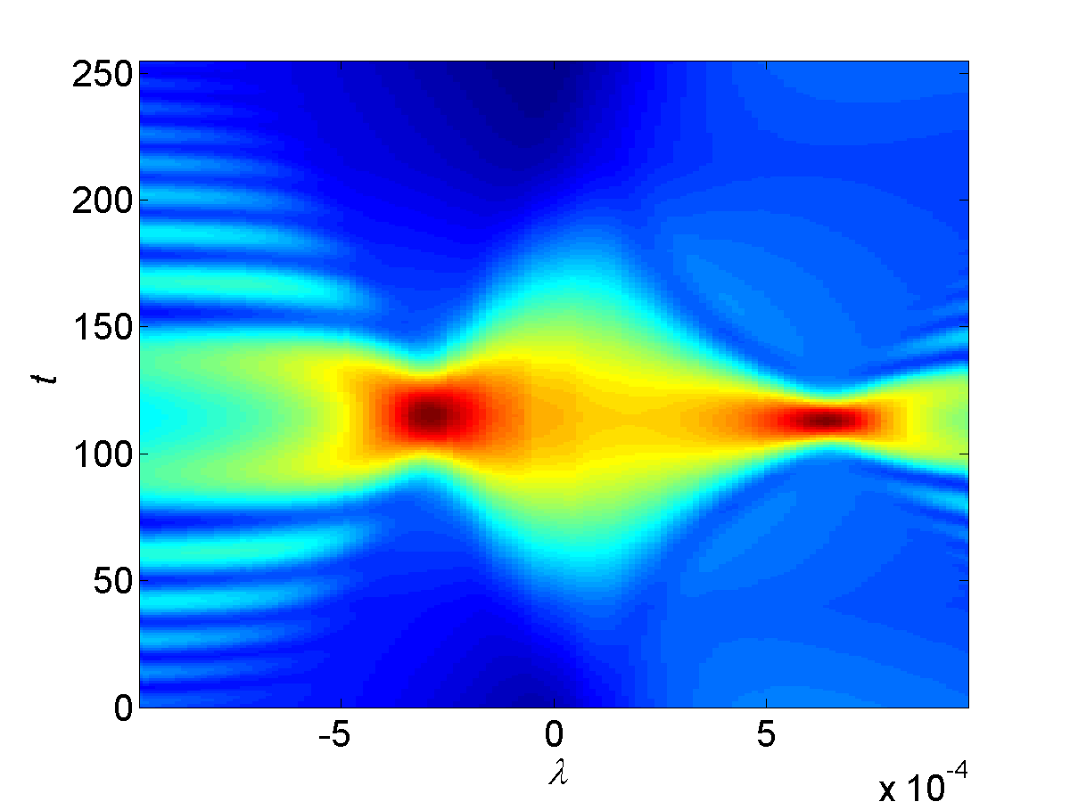
Consider again the signal in (39), Figure 5 shows the slices of the filter-matched CT defined by (40) with Gaussian window and (discrete points, unitless). Observe that by comparing the corresponding pictures in Figure 4 and Figure 5, the filter-matched CT indeed improves the separability of the two components when their IFs are crossover.
For , we will use the filter-matched CT to estimate by
| (41) |
with
| (42) |
where is defined in Theorem 1. We call the ridge of the filter-matched CT.
With the resulting , we may use the CT (namely (33) or (34)) to recover sub-signal . Observe that the recovering formula (33) or (34) recovers one by one. Next, by considering all as a whole group, we propose an innovative algorithm based on the filter-matched CT to recover sub-signals .
Recall that when is the Gaussian window given in (23), then (38) holds. Thus for , we have
Hence if obtained from the filter-matched CT by (42) are good approximations to , then, with , we have
In particular, with , we have
| (43) |
where
| (44) |
Denote
| (45) |
Then (43) can be written as
Hence
| (46) |
Based (46), we propose the following algorithm, called the group filter-matched chirplet transform-based signal separation scheme (GFCT3S), to recover components and trend .
Algorithm 1.
We first apply the CT to the blind source signal , with output for thresholding with the appropriate parameter that can be determined by the energy distribution of . This allows us to separate the thresholded set into different clusters . Note that is a fast decay function with respect to . If all the sub-signals are well-separated in the time-frequency plane, namely satisfy (2), then for , and hence, in (47) is essentially the identity matrix. So the reconstruction algorithm above is fit for both cases in (2) and (3).
Finally, we discuss the algorithm of real-time processing of an consecutive input signal. To reduce the computational cost, we need to predefine some variables. Let denote the truncation length of the input signal, e.g. or , then frequency is discretized into and is discretized into . Define , where is a fixed time. Suppose we will separate when , then we need to calculate first, where should equivalent to the window length in (40) and . Then for the next time instant , we just need to calculate , and continue the procedure.


|


|

|
.
4 Numerical experiments
Figure 2 demonstrates our proposed method GFCT3S (Algorithm 1) is efficient for the two-component signal in (13) with one cross point of the IFs. In this section, we first consider another synthetic multicomponent signal , given as
| (48) |
where . Note that the IFs of and are and , respectively, called IF1 and IF2 in Figure 7.
In this experiment, we discretize with a sampling rate kHz and data length , namely . Figure 6 shows the waveform of and the IFs of two AM-FM components, and . As the expression in (48), consists of one trend and two oscillating AM-FM components. Meanwhile, the IFs of the two AM-FM components are crossover.
Observe that the signal to be processed contains lots of samples, which should be analyzed or separated locally. Here we use a sliding truncated Gaussian window with length of points for methods of STFT, SST and GFCT3S. Hence the frequency bins is discretized as for complex signals, or just for real signals. Note that we set as a power of 2 to take full advantage of the fast Fourier transform. Figure 7 shows the time-frequency diagrams of the STFT and the 2nd-order SST in [38] and the recovered IFs by the ridges of the filter-matched CT given in (42). The enlarged pictures around are also attached with each sub-Figure. Obviously, when the IFs of and are crossover, either the STFT or the 2nd-order SST hardly represents the sub-signals reliably. Thus we cannot use the time-frequency diagram of the STFT or the 2nd-order SST to extract the IFs of the sub-signals for the purpose of recovering their waveforms. However, using the ridges of the filter-matched CT, we can extract the IFs of accurately.

|


|

|
|
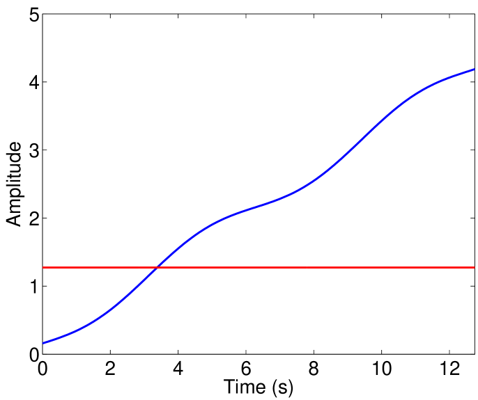
Figure 8 provides recovered modes and around with GFTC3S (Algorithm 1) proposed in Section 3.2. Since there are so many sample periods of the signal , we just show a small truncation around . Observe the differences between the recovered waveforms and the truth ones are extremely small.
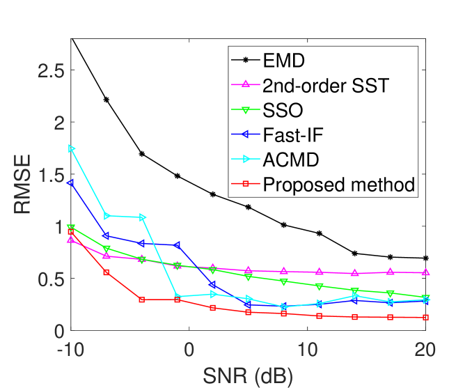
To demonstrate the efficiency of our computational scheme for signal data with additive noise, we compared the proposed algorithm with the following methods: EMD [1], 2nd-order SST [38], SSO [48], Fast-IF [60], and ACMD [66]. Among these algorithms, Fast-IF, and ACMD are the ones that take crossover frequencies into account. To measure the errors, we use the root-mean-square error (RMSE) defined by
where is the estimation of a function . The left panel of Figure 9 provides the RMSEs of and when signal-to-noise ratios (SNRs) vary from dB to dB. Note that the recovery performance tends to be stationary when SNR is larger than 0dB. From the right panel of Figure 9, where the average RMSE is defined by , we find that the existing methods EMD and 2nd-order SST and SSO are hardly to recover the sub-signals and with crossover IFs. Our method outperforms Fast-IF and ACMD. As shown in this figure, our algorithm posses the best stability with respect to robustness.

|

|

|

|

|

|

|

|
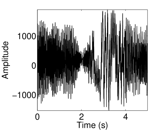
Finally, we consider a real signal, the radar echoes. Figure 10 shows the waveform and spectrum of the radar echoes. Note that the sampling rate here is equal to 400 Hz, which is just the pulse repetition frequency of the radar. The bottom panel of Figure 10, namely the spectrum shows that this signal consists of several broadband components and a trend.
Figure 11 shows some results of the radar echoes given in Figure 10. From their STFTs (top-left panel in Figure 11), there are two components (two radar targets) in the echoes. Meanwhile, the IF curves of these two targets are crossover with the trend component. Although the 2nd-order SST can squeeze the time-frequency plane of STFT, it is still affected by the trend component when they are crossover. The top-right panel of Figure 11 shows a specific slice of 3D filter-matched CT matrix, where the chirp rate is close to those of Component 1 and Component 2. Observe that in this specific slice, compared with STFT and 2nd-order SST, the two signal components are enhanced a lot. The left-bottom panel shows the estimated IFs by the ridges of filter-matched CT given in (42). The recovered waveforms of Component 1 (real part) and Component 2 (real part) by GFCT3S are provided in the middle and right panels in the bottom row of Figure 11.
5 Conclusions
In this paper, we propose a method based the chirplet transform (CT) to retrieve modes of multicomponent signals with crossover instantaneous frequencies. We define the modified adaptive harmonic model and the conditions to represent crossover components separately by the proposed CT-based method. The error bounds for instantaneous frequency estimation and sub-signal recovery are provided. Based on the approximation of source signals with linear chirps at any local time, we propose an improved CT-based signal reconstruction algorithm with all signal components taken into account. The numerical experiments demonstrate the proposed method are more accurate and consistent in signal separation than EMD, SST, SSO and other approaches such as Fast-IF and ACMD. The proposed method has a great potential for a variety of engineering applications such as channel detection in communication, fault monitoring in mechanical systems, radar signal processing etc.
Appendix
In following, as in Theorem 1. In addition, since in general is small, we assume for simplicity of presentation. Furthermore, since will be fixed throughout the proof, in the following we use , , and to denote , , and respectively. First we establish a few lemmas.
Lemma 1.
For , let be the linear chirp approximation to at time defined above. Then
| (51) |
Lemma 2.
For , let be its transform by CT and be the approximation of with linear chirps defined by (49). Then
| (52) |
Proof.
Lemma 3.
Let be the sets defined by (27). If , then are nonoverlapping, namely, for .
Proof.
Assume for some . By the definition of , we have
a contradiction to the well-separated condition (3). Thus the sets are nonoverlapping. ∎
Since we assume , from (3), we have
| (53) |
Lemma 4.
Proof.
Proof of Theorem (a). Let . Suppose for any . Then
Hence,
This, together with (52), implies
where the second last inequality follows (26) on the condition for . This leads to a contradiction that . Hence there must exist such that . Lemma 3 has shown that are disjoint.
Finally we show that each is non-empty. To this regard, we show . Indeed, the following fact followed from (55)
implies
Hence .
Acknowledgments
The authors thank the anonymous reviewers for their valuable comments.
This work was partially supported by the ARO under Grant W911NF2110218, HKBU Grant RC-FNRA-IG/18-19/SCI/01, the Simons Foundation under Grant 353185, the National Natural Science Foundation of China under Grants 62071349.
References
- [1] N.E. Huang, Z. Shen, S.R. Long, M.L. Wu, H.H. Shih, Q. Zheng, N.C. Yen, C.C. Tung, and H.H. Liu, “The empirical mode decomposition and Hilbert spectrum for nonlinear and nonstationary time series analysis,” Proc. Roy. Soc. London A, vol. 454, no. 1971, pp. 903–995, Mar. 1998.
- [2] P. Flandrin, G. Rilling, and P. Goncalves, “Empirical mode decomposition as a filter bank,” IEEE Signal Proc. Letters, vol. 11, no. 2, pp. 112–114, Feb. 2004.
- [3] N. Ur Rehman and D. P. Mandic, “Filter bank property of multivariate empirical mode decomposition,” IEEE Trans. Signal Proc., vol. 59, no. 5, pp. 2421-2426, May 2011.
- [4] G. Rilling and P. Flandrin, “One or two frequencies? The empirical mode decomposition answers,” IEEE Trans. Signal Proc., vol. 56, pp. 85–95, Jan. 2008.
- [5] Z. Wu and N.E. Huang, “Ensemble empirical mode decomposition: A noise-assisted data analysis method,” Adv. Adapt. Data Anal., vol. 1, no. 1, pp. 1–41, Jan. 2009.
- [6] Y.S. Xu, B. Liu, J. Liu, and S. Riemenschneider, “Two-dimensional empirical mode decomposition by finite elements,” Proc. Roy. Soc. London A, vol. 462, no. 2074, pp. 3081–3096, Oct. 2006.
- [7] L. Lin, Y. Wang, and H.M. Zhou, ”Iterative filtering as an alternative algorithm for empirical mode decomposition,” Adv. Adapt. Data Anal., vol. 1, no. 4, pp. 543–560, Oct. 2009.
- [8] N. Ur Rehman and D.P. Mandic, “Empirical mode decomposition for trivariate signals,” IEEE Trans. Signal Proc., vol. 58, no. 3, pp. 1059-68, Mar. 2010.
- [9] T. Oberlin, S. Meignen, and V. Perrier, “An alternative formulation for the empirical mode decomposition,” IEEE Trans. Signal Proc., vol. 60, no. 5, pp. 2236–2246, May 2012.
- [10] Y. Wang, G.-W. Wei and S.Y. Yang , “Iterative filtering decomposition based on local spectral evolution kernel,” J. Scientific Computing, vol. 50, no. 3, pp. 629–664, Mar. 2012.
- [11] A. Cicone, J.F. Liu, and H.M. Zhou, “Adaptive local iterative filtering for signal decomposition and instantaneous frequency analysis,” Appl. Comput. Harmon. Anal., vol. 41, no. 2, pp. 384–411, Sep. 2016.
- [12] J. Gilles, “Empirical wavelet transform,” IEEE Trans. Signal Proc., vol. 61, no. 16, pp. 3999-4010, Aug. 2013.
- [13] L. Li, H.Y. Cai, Q.T. Jiang and H.B. Ji, “An empirical signal separation algorithm for multicomponent signals based on linear time-frequency analysis,” Mechanical Systems and Signal Proc., vol. 121, no. 4, pp. 791–809, Apr. 2019.
- [14] M.D. van der Walt, “Empirical mode decomposition with shape-preserving spline interpolation,”Results in Appl. Math., vol. 5, 100086, Feb. 2020.
- [15] L. Li and H.B. Ji, “Signal feature extraction based on improved EMD method,” Measurement, vol. 42, pp. 796–803, Jun. 2009.
- [16] L. Cohen, Time-frequency Analysis, Prentice Hall, New Jersey, 1995.
- [17] H. Hassanpour, M. Mesbah and B. Boashash, “SVD-based TF feature extraction for newborn EEG seizure,” EURASIP Journal on Advances in Signal Proc., vol. 16, pp. 2544–2554, 2004.
- [18] L. Stankovi, T. Thayaparan, and M. Dakovi, “Signal decomposition by using the S-method with application to the analysis of HF radar signals in sea-clutter,” IEEE Trans. Signal Proc., vol. 54, no. 11, pp. 4332–4342, Nov. 2006.
- [19] L. Stankovi, D. Mandi, M. Dakovi, and M. Brajovi, “Time-frequency decomposition of multivariate multicomponent signals,” Signal Proc., vol. 142, pp. 468–479, Jan. 2018.
- [20] I. Daubechies, J.F. Lu, and H.-T. Wu, “Synchrosqueezed wavelet transforms: An empirical mode decomposition-like tool,” Appl. Computat. Harmon. Anal., vol. 30, no. 2, pp. 243–261, Mar. 2011.
- [21] I. Daubechies and S. Maes, “A nonlinear squeezing of the continuous wavelet transform based on auditory nerve models,” in A. Aldroubi, M. Unser Eds. Wavelets in Medicine and Biology, CRC Press, 1996, pp. 527-546.
- [22] G. Thakur and H.-T. Wu, “Synchrosqueezing based recovery of instantaneous frequency from nonuniform samples,” SIAM J. Math. Anal., vol. 43, pp. 2078–2095, 2011.
- [23] H.-T. Wu, Adaptive Analysis of Complex Data Sets, Ph.D. dissertation, Princeton Univ., Princeton, NJ, 2012.
- [24] T. Oberlin, S. Meignen, and V. Perrier, “The Fourier-based synchrosqueezing transform,” in Proc. 39th Int. Conf. Acoust., Speech, Signal Process. (ICASSP), 2014, pp. 315–319.
- [25] S. Meignen, T. Oberlin, and S. McLaughlin, “A new algorithm for multicomponent signals analysis based on synchrosqueezing: With an application to signal sampling and denoising,” IEEE Trans. Signal Proc., vol. 60, no. 11, pp. 5787–5798, Nov. 2012.
- [26] F. Auger, P. Flandrin, Y. Lin, S.McLaughlin, S. Meignen, T. Oberlin, and H.-T. Wu, “Time-frequency reassignment and synchrosqueezing: An overview,” IEEE Signal Process. Mag., vol. 30, no. 6, pp. 32–41, Nov. 2013.
- [27] C. Li and M. Liang, “Time frequency signal analysis for gearbox fault diagnosis using a generalized synchrosqueezing transform,” Mechanical Systems and Signal Proc., vol. 26, pp. 205–217, Jan. 2012.
- [28] S.B. Wang, X.F. Chen, I.W. Selesnick, Y.J. Guo, C.W. Tong and X.W. Zhang, “Matching synchrosqueezing transform: A useful tool for characterizing signals with fast varying instantaneous frequency and application to machine fault diagnosis,” Mechanical Systems and Signal Proc., vol. 100, pp. 242–288, Feb. 2018.
- [29] H.Z. Yang, J.F. Lu, and L.X. Ying, “Crystal image analysis using 2D synchrosqueezed transforms,” Multiscale Modeling Simulation, vol. 13, no. 4, pp. 1542–1572, 2015.
- [30] J.F. Lu and H.Z. Yang, “Phase-space sketching for crystal image analysis based on synchrosqueezed transforms,” SIAM J. Imaging Sci., vol. 11, no. 3, pp.1954–1978, 2018.
- [31] K. He, Q. Li, and Q. Yang, “Characteristic analysis of welding crack acoustic emission signals using synchrosqueezed wavelet transform,” J. Testing and Evaluation, vol. 46, no. 6, pp. 2679–2691, 2018.
- [32] H.-T. Wu, Y.-H. Chan, Y.-T. Lin, and Y.-H. Yeh, “Using synchrosqueezing transform to discover breathing dynamics from ECG signals,”Appl. Comput. Harmon. Anal., vol. 36, no. 2, pp. 354–459, Mar. 2014.
- [33] H.-T. Wu, R. Talmon, and Y.L. Lo, “Assess sleep stage by modern signal processing techniques,” IEEE Trans. Biomedical Engineering, vol. 62, no. 4, 1159–1168, 2015.
- [34] C. L. Herry, M. Frasch, A. J. Seely1, and H. -T. Wu, “Heart beat classification from single-lead ECG using the synchrosqueezing transform,” Physiological Measurement, vol. 38, no. 2, Jan. 2017.
- [35] S. Wang, X. Chen, G. Cai, B. Chen, X. Li, and Z. He, “Matching demodulation transform and synchrosqueezing in time-frequency analysis,” IEEE Trans. Signal Proc., vol. 62, no. 1, pp. 69–84, 2014.
- [36] Q.T. Jiang and B.W. Suter, “Instantaneous frequency estimation based on synchrosqueezing wavelet transform,” Signal Proc., vol. 138, no.9, pp.167–181, 2017.
- [37] C. Li and M. Liang, “A generalized synchrosqueezing transform for enhancing signal time-frequency representation,” Signal Proc., vol. 92, no. 9, pp. 2264–2274, 2012.
- [38] T. Oberlin, S. Meignen, and V. Perrier, “Second-order synchrosqueezing transform or invertible reassignment? towards ideal time-frequency representations,” IEEE Trans. Signal Proc., vol. 63, no. 5, pp.1335–1344, Mar. 2015.
- [39] T. Oberlin and S. Meignen, “The 2nd-order wavelet synchrosqueezing transform,” in 2017 IEEE International Conference on Acoustics, Speech and Signal Processing (ICASSP), March 2017, New Orleans, LA, USA.
- [40] D.H. Pham and S. Meignen, “High-order synchrosqueezing transform for multicomponent signals analysis- With an application to gravitational-wave signal,” IEEE Trans. Signal Proc., vol. 65, no. 12, pp.3168–3178, Jun. 2017.
- [41] L. Li, Z.H. Wang, H.Y. Cai, Q.T. Jiang, and H.B. Ji, “Time-varying parameter-based synchrosqueezing wavelet transform with the approximation of cubic phase functions,” in 2018 14th IEEE Int’l Conference on Signal Proc. (ICSP), pp. 844–848, Aug. 2018.
- [42] L. Li, H.Y. Cai, H.X. Han, Q.T. Jiang and H.B. Ji, “Adaptive short-time Fourier transform and synchrosqueezing transform for nonstationary signal separation,” Signal Proc., vol. 166, 2020, 107231.
- [43] L. Li, H.Y. Cai, and Q.T. Jiang, “Adaptive synchrosqueezing transform with a time-varying parameter for nonstationary signal separation,” Appl. Comput. Harmon. Anal., vol. 49, 1075–1106, 2020.
- [44] J. Lu, Q.T. Jiang and L. Li, “Analysis of adaptive synchrosqueezing transform with a time-varying parameter,” Advances in Comput. Math., vol. 46, 2020, Article number: 72.
- [45] H.Y. Cai, Q.T. Jiang, L. Li, and B.W. Suter, “Analysis of adaptive short-time Fourier transform-based synchrosqueezing transform,” Analysis and Applications, vol. 19, no. 1, pp. 71–105, 2021.
- [46] Y.-L. Sheu, L.-Y. Hsu, P.-T. Chou, and H.-T. Wu, “Entropy-based time-varying window width selection for nonlinear-type TF analysis,” Int’l J. Data Sci. Anal., vol. 3, pp. 231–245, 2017.
- [47] A. Berrian and N. Saito, “Adaptive synchrosqueezing based on a quilted short-time Fourier transform,” arXiv:1707.03138v5, Sep. 2017.
- [48] C.K. Chui and H.N. Mhaskar, “Signal decomposition and analysis via extraction of frequencies,” Appl. Comput. Harmon. Anal., vol. 40, no. 1, pp. 97–136, 2016.
- [49] C.K. Chui and N.N. Han, “Wavelet thresholding for recovery of active sub-signals of a composite signal from its discrete samples,” Appl. Comput. Harmon. Anal., vol. 52, pp. 1–24, 2021.
- [50] C.K. Chui, Q.T. Jiang, L. Lin, and J. Lu, “Signal separation based on adaptive continuous wavelet-like transform and analysis,” Appl. Comput. Harmon. Anal., vol. 53, pp. 151–179, 2021.
- [51] L. Li, C.K. Chui, and Q.T. Jiang, “Direct signals separation via extraction of local frequencies with adaptive time-varying parameters,” preprint, 2020. arXiv2010.01866v1
- [52] C.K. Chui, Q.T. Jiang, L. Li, and J. Lu, “Analysis of an adaptive short-time Fourier transform-based multicomponent signal separation method derived from linear chirp local approximation”, Journal of Comput. & Appl. Math., vol. 382, 2021, 113074.
- [53] V.C. Chen, F. Li, S.-S. Ho, and H. Wechsler, “Micro-Doppler effect in radar : phenomenon, model, and simulation study,” IEEE Trans. Aerosp. Electron. Syst., vol. 42, no. 1, pp. 2–21, 2006.
- [54] L. Stankovi, I. Orovi, S. Stankovi, and M. Amin, “Compressive sensing based separation of nonstationary and stationary signals overlapping in time-frequency,” IEEE Trans. Signal Proc., vol 61, no. 18, pp. 4562–4572, Sep. 2013.
- [55] P. Li, and Q.H. Zhang, “IF estimation of overlapped multicomponent signals based on viterbi algorithm,” Circuits, Syst., Signal Process., vol 39, no. 6, pp. 3105-3124, 2020.
- [56] X.X. Zhu, H.Z. Yang, Z.S. Zhang, J.H. Guo, and N.H. Liu, “Frequency-chirprate reassignment,” Digit. Signal Process., vol 104, 102783, Jun. 2020.
- [57] V. Bruni, M. Tartaglione, and D. Vitulano,“Radon spectrogram-based approach for automatic IFs separation,” EURASIP J. Adv. Signal Process., pp. 1-21, Mar. 2020.
- [58] V. Bruni, M. Tartaglione, and D. Vitulano,“A pde-based analysis of the spectrogram image for instantaneous frequency estimation,” Mathematics, vol. 9, no. 3, pp. 3105-3124, Jan. 2021.
- [59] I. Djurovi,“QML-RANSAC instantaneous frequency estimator for overlapping multicomponent signals in the time-frequency plane,” IEEE Signal Proc. Letters, vol. 25, no. 3 447-451, Mar. 2018.
- [60] N.A. Khan and S. Ali,“A robust and efficient instantaneous frequency estimator of multi-component signals with intersecting time-frequency signatures,” Signal Proc., vol. 177, 107728, Dec. 2020.
- [61] Y. Yang, X. J. Dong, Z. K. Peng, W. M. Zhang, and G. Meng,“Component extraction for non-stationary multi-component signal using parameterized de-chirping and band-pass filter,”IEEE Signal Proc. Letters, vol. 22, no. 9, 1373-1377, Sep. 2014.
- [62] S. Chen, X. Dong, G. Xing, Z. Peng, W. Zhang, and G. Meng, “Separation of overlapped non-stationary signals by ridge path regrouping and intrinsic chirp component decomposition,” IEEE Sensors Journals, vol. 17, no. 18, pp. 5994–6005, Sep. 2017.
- [63] B. Barkat and K. Abed-Meraim, “Algorithms for blind components separation and extraction from the time-frequency distribution of their mixture,” EURASIP J. Appl. Signal Proc., vol. 13, pp. 2025–2033, 2004.
- [64] S. Chen, Z. Peng, Y.Yang, X. Dong, and W. Zhang, “Intrinsic chirp component decomposition by using Fourier Series representation,” Signal Proc., vol. 137, pp. 319–327, Feb. 2017.
- [65] O. Chen, X. Lang, L. Xie, and H. Su, “Multivariate intrinsic chirp mode decomposition,” Signal Proc., vol. 183, Jan. 2021.
- [66] S. Chen, X. Dong, Z. Peng, W. Zhang, and G. Meng, “Nonlinear Chirp Mode Decomposition: A Variational Method,” IEEE Trans. Signal Proc., vol. 65, no. 22, pp. 6024–6037, Nov. 2017.
- [67] P. Zhou, Y. Yang, S. Chen, Z. Peng, K. Noman, and W.Zhang, “Parameterized model based blind intrinsic chirp source separation,” Digit. Signal Process., vol 83, pp. 73-82, Aug. 2018.
- [68] Z. Liu, Q. He, S. Chen, X. Dong, Z. Peng, and W. Zhang, “Frequency-domain intrinsic component decomposition for multimodal signals with nonlinear group delays,” Signal Proc., vol. 154, pp. 57-63. 2019.
- [69] S. Q. Chen, Y. Yang, Z.Peng, X. J. Dong, W. Zhang, and G. Meng, “Adaptive chirp mode pursuit: Algorithm and applications,” Mechanical Systems and Signal Proc., vol. 116, pp. 566–584, Feb. 2019.
- [70] L. Stankovi, M. Dakovi, T.Thayaparan, and V. Bugarin, “Inverse radon transform-based micro-doppler analysis from a reduced set of observations,” IEEE Trans. Aerosp. Electron. Syst., vol. 51, no. 2, pp. 1155–1169, Feb. 2015.
- [71] S. Mann and S. Haykin, “The chirplet transform: Physical considerations,” IEEE Trans. Signal Proc., vol. 43, no. 11, pp. 2745–2761, Nov. 1995.
- [72] R. G. Baraniuk, and D. L. Jones, “Wigner-based formulation of the chirplet transform,” IEEE Trans. Signal Proc., vol. 44, no. 12, pp. 3129–3135, Dec. 1996.
- [73] J. Zheng J, H. Liu, and Q. Liu, “Parameterized centroid frequency-chirp rate distribution for LFM signal analysis and mechanisms of constant delay introduction,” IEEE Trans. Signal Proc., vol. 65, no. 24, pp. 6435–6447, Dec. 2017.
- [74] K. Czarnecki, D. Fourer, F. Auger, and M. Rojewski, “A fast time-frequency multi-window analysis using a tuning directional kernel,” Signal Proc., vol. 147, pp. 110–119, Jun. 2018.
- [75] V. Katkovnik, “A new form of the Fourier transform for time-frequency estimation,” Signal Proc., vol. 47, no. 2, pp. 187–200, 1995.
- [76] X. Li, G. Bi, S. Stankovi, and A.M. Zoubir, “Local polynomial Fourier transform: A review on recent developments and applications,” Signal Proc., vol. 91, no.6, pp.1370–1393, 2011.
- [77] L. Stankovi, M. Dakovi, and T. Thayaparan, Time-Frequency Signal Analysis with Applications, Artech House, Boston, 2013.
- [78] G. Beylkin, “Discrete radon transform,” IEEE Trans. Acoust. Speech Signal Process., vol. 35, no. 2, pp. 162-172, Feb. 1987.
- [79] A. Averbuch and Y. Shkolnisky, “3D Fourier based discrete Radon transform,” Appl. Comput. Harmon. Anal., vol. 15, pp. 33–69, July 2003.
- [80] M. Wang, A.K. Chan, and C.K. Chui, “Linear frequency-modulated signal detection using Radon-ambiguity transform,” IEEE Trans. Signal Proc., vol. 46, no. 3, pp. 571-586, Mar. 1998.