A characterization of constant -mean curvature surfaces in the Heisenberg group
Abstract.
In Euclidean -space, it is well known that the Sine-Gordon equation was considered in the nineteenth century in the course of investigations of surfaces of constant Gaussian curvature . Such a surface can be constructed from a solution to the Sine-Gordon equation, and vice versa. With this as motivation, employing the fundamental theorem of surfaces in the Heisenberg group , we show in this paper that the existence of a constant -mean curvature surface (without singular points) is equivalent to the existence of a solution to a nonlinear second-order ODE (1.2), which is a kind of Liénard equations. Therefore, we turn to investigate this equation. It is a surprise that we give a complete set of solutions to (1.2) (or (1.5)), and hence use the types of the solution to divide constant -mean curvature surfaces into several classes. As a result, after a kind of normalization, we obtain a representation of constant -mean curvature surfaces and classify further all constant -mean curvature surfaces. In Section 9, we provide an approach to construct -minimal surfaces. It turns out that, in some sense, generic -minimal surfaces can be constructed via this approach. Finally, as a derivation, we recover the Bernstein-type theorem which was first shown in [3] (or see [7, 8]).
Key words and phrases:
Keywords: Heisenberg group, Pansu sphere, p-Minimal surface, Liénard equation, Bernstein theorem1991 Mathematics Subject Classification:
1991 Mathematics Subject Classification. Primary: 53A10, 53C42, 53C22, 34A26.1. Introduction and main results
In literature, the Heisenberg group and its sub-Laplacian are active in many fields of analysis and sub-Riemannian geometry, control theory, semiclassical analysis of quantum mechanics, etc. (cf. [18, 19, 20, 21, 22]). It also has applications in signal analysis and geometric optics [31, 32, 33]. Research on the sub-Riemannian geometry and its analytical consequences, in particular geodesics, has been studied widely and extensively in the past ten years (cf. [19, 23, 24, 25, 26, 27, 29, 28, 30]). In this paper, the Heisenberg group is studied as a pseudo-hermitian manifold. Like Euclidean geometry, it is a branch of Klein geometries, and the corresponding Cartan geometry is pseudo-hermitian geometry.
Recall that the Heisenberg group is the space associated with the group multiplication
which is a -dimensional Lie group. The space of all left invariant vector fields is spanned by the following three vector fields:
The standard contact bundle on is the subbundle of the tangent bundle which is spanned by and . It is also defined to be the kernel of the contact form
The CR structure on is the endomorphism defined by
One can view as a pseudo-hermitian manifold with as the standard pseudo-hermitian structure. There is a natural associated connection if we regard all these left invariant vector fields and as parallel vector fields. A naturally associated metric on is the adapted metric , which is defined by . It is equivalent to define the metric by regarding and as an orthonormal frame field. We sometimes use to denote the adapted metric. In this paper, we use the adapted metric to measure the lengths and angles of vectors, and so on.
A pseudo-hermitian transformation (or a Heisenberg rigid motion) in is a diffeomorphism in which preserves the standard pseudo-hermitian structure . We let be the group of Heisenberg rigid motions, that is, the group of all pseudo-hermitian transformations in . For details of this group, we refer readers to [4, 6], in which the fundamental theorem in the Heisenberg groups has been studied. We say that two surfaces are congruent if they differ by an action of a Heisenberg rigid motion.
The concept of minimal surfaces or constant mean curvature surfaces plays an important role in differential geometry to study the basic properties of manifolds. There is an analogous concept in pseudo-hermitian manifolds, which are called -minimal surfaces. In this paper, we focus on studying such kinds of surfaces in the Heisenberg group . Throughout this article, all objects we discuss are assumed to be smooth, unless we specify otherwise. Suppose is a surface in the Heisenberg group . There is a one-form on which is induced from the adapted metric . This induced metric is defined on the whole surface and is called the first fundamental form of . The intersection is integrated to be a singular foliation on called the characteristic foliation. Each leaf is called a characteristic curve. A point is called a singular point if at which the tangent plane coincides with the contact plane ; otherwise, is called a regular (or non-singular) point. Generically, a point is a regular point, and the set of all regular points is called the regular part of . On the regular part, we can choose a unit vector field such that defines the characteristic foliation. The vector is determined up to a sign. Let . Then forms an orthonormal frame field of the contact bundle . We usually call the vector field a horizontal vector field. Then the -mean curvature of the surface is defined by
| (1.1) |
The -mean curvature is only defined on the regular part of . There are two more equivalent ways to define the -mean curvature from the point of view of variation and a level surface (see [3, 34]). We remark that this notion of mean curvature was proposed by J.-H. Cheng, J.-F. Hwang, A. Malchiodi, and P. Yang from the geometric point of view to generalize the one introduced first by S. Pauls in for graphs over the -plane [35]. Also, in [36], M. Ritoré and C. Rosales exposed another method to compute the mean curvature of a hypersurface. If on the whole regular part, we call the surface a -minimal surface. The -mean curvature is the line curvature of a characteristic curve, and hence the characteristic curves are straight lines (for the detail, see [3]). There also exists a function defined on the regular part such that is tangent to the surface . We call this function the -function of . It is uniquely determined up to a sign, which depends on the choice of the characteristic direction . Define and , then forms an orthonormal frame field of the tangent bundle . Notice that is uniquely determined and independent of the choice of the characteristic direction . In [6], it was shown that these four invariants,
form a complete set of invariants for surfaces in . We remark that all the results provided in [6] still hold in the -category. For each regular point , we can choose suitable coordinates around to study the local geometry of such surfaces. There always exists a coordinate system of such that
We call such coordinates a compatible coordinate system. It is determined up to a transformation in (2.19). Notice that the compatible coordinate systems are dependent on the characteristic direction .
Let be a constant -mean curvature surface with . In terms of a compatible coordinate system , the -function satisfies the following equation
| (1.2) |
which first appeared as a Codazzi-like equation in [4] with .
It is a nonlinear ordinary differential equation and is an example of the so-called Liénard equations, named after the French physicist Alfred-Marie Liénard. The Liénard equations were intensely studied as they can be used to model oscillating circuits. Conversely, in this paper, we show that if there exists a solution to the Liénard equation (1.2), we are able to construct a constant -mean curvature surface with and this given solution as its -function. This result is summarized as Theorem 1.1. One motivation of this theorem comes from the famous Sine-Gordon Equation (SGE),
which is considerably older than the Korteweg de Vries Equation (KdV). It was discovered in the late eighteenth century in the study of pseudospherical surfaces, that is, surfaces of Gaussian curvature immersed in , and it was intensively studied for this reason. It arises from the Gauss-Codazzi equations for pseudospherical surfaces in and is known as an integrable equation [13]. In addition, it can also be viewed as a continuum limit [14]. Its solutions and solitons have been widely discussed by the Inverse Scattering Transform and other approaches.
There is a bijective relation between solutions of the SGE with and the classes of pseudospherical surfaces in up to rigid motion. If is a solution such that is zero at a point , then the immersed pseudoshperical surface has cusp singularities. For example, the pseudospherical surfaces corresponding to the 1-soliton solutions of SGE are the so-called Dini surfaces and have a helix of singularities.
The study of line congruences gives rise to the concept of Bäcklund transformations. A line congruence is called a Bäcklund transformation with the constant angle between the normal to at and the normal to at and the distance between and is for all . The classical Bäcklund transformation for the Sine-Gordon equation was constructed in the nineteenth century by Swedish differential geometer Albert Bäcklund by means of a geometric construction [15, 16, 17]. We then are motivated to present analogous theorems for Heisenberg groups.
Theorem 1.1.
The existence of a constant -mean curvature surface without singular points in is equivalent to the existence of a solution to the equation (1.2). More precisely, let and be two arbitrary smooth functions on a coordinate neighborhood . If they satisfy the following integrability condition
| (1.3) |
for some functions and in the variable , then there exists an embedding provided that is small enough such that the surface has and as its -mean curvature and -function, respectively, and , with and defined as (2.15) and (2.18). In addition, such embeddings are unique, up to a Heisenberg rigid motion.
In this article, we sometimes call the Liénard equation (1.2) as the Codazzi-like equation from the geometrical point of view [4, 6]. We would also like to specify that a graph is -minimal if it satisfies the -minimal equation (see [3])
| (1.4) |
This is a degenerate hyperbolic and elliptic partial differential equation.
Theorem 1.1 is the fundamental theorem for surfaces in . After we make a detailed investigation of the original version of the integrability conditions (2.1), (1.3) is more useful than the previous one in some sense (for the origin version, we refer readers to [6] or Theorem 2.1 of this paper). It also appeared as Theorem H in [4] with a slightly different formulation as the authors of [4] did not prescribe the metric.
Theorem 1.1 follows from our detailed study on the integrability condition (see (2.1)) of the fundamental theorem (Theorem 2.1) for surfaces in . Actually, if we let be the Levi-Civita connection associated to the induced metric with respect to the orthonormal frame field , as specified in Theorem 1.1, then (1.3) means that , and satisfy the integrability condition (2.1). This is equivalent to saying that and satisfy the integrability condition (2.13) (see Subsection 2.2), which is another version of (2.1). We then have Theorem 1.1.
Given a function in a coordinate neighborhood which satisfies the Codazzi-like equation (1.2), we are able to construct a family of constant -mean curvature surfaces. Therefore, it suggests that a good strategy is to investigate constant -mean curvature surfaces by means of the Codazzi-like equation (1.2); in particular, -minimal surfaces. In this paper, we will focus on the theory of -minimal surfaces. Strategically, we first study the equation (1.2) with , that is,
| (1.5) |
For nonlinear ordinary differential equations, it is known that it is rarely possible to find explicit solutions in closed form, even in power series. Fortunately, we indeed obtain a complete set of solutions to (1.5) in a simple form (see Section 4), stated as follows.
Theorem 1.2.
In Subsection 5.1, we are able to use the types of the solutions in Theorem 1.2 to divide the -minimal surfaces into several classes, which are vertical, special type I, special type II and general type (see Definition 5.1 and 5.2). Each type of these -minimal surfaces is open and contains no singular points. Generically, each -minimal surface is a union of these types of surfaces, and ”type” can be shown to be invariant under an action of a Heisenberg rigid motion. Now for each type, whether it is special or general, if a function is given, then Proposition 5.3, 5.4 and 5.5 express the formula for the induced metric (see (5.5), (5.6) and (5.7)), which is a representation of , on the -minimal surfaces with this given as -function. From these formulae, we see that such constructed -minimal surfaces depend upon two functions and for each given . Nonetheless, in Section 6, we proceed to normalize these invariants to the following normal forms in terms of an orthogonal coordinate system , which is a coordinate system such that . Such a coordinate system is determined up to a translation on , thus we call it a normal coordinate system.
Theorem 1.3.
Let be a -minimal surface. Then, in terms of a normal coordinate system , we can normalize the -function and the induced metric to be the following normal forms:
-
(1)
, and if is of special type I,
-
(2)
, and if is of special type II,
-
(3)
, and if is of general type,
for some functions and , in which is unique up to a translation on , and is unique up to a translation on as well as its image.
Therefore, constitutes a complete set of invariants for -minimal surfaces of special type I (or of special type II), whereas both and constitute a complete set of invariants for -minimal surfaces of general type. We hence give a representation for -minimal surfaces (see Section 6). From Theorem 1.3, together with Theorem 1.1, the following version of the fundamental theorem holds immediately for -minimal surfaces in .
Analogs for constant -mean curvature surfaces are also included in Subsection 5.2. We first derive the general form of to the Codazzi-like equation (1.2) for ( stated as Theorem 1.4), and Proposition 5.6 provides the formula for the induced metric and .
Theorem 1.4.
Besides the trivial solution , the Codazzi-like equation (1.2) for nonzero has the special solutions
and the general solution of the form
| (1.7) |
which depends on two constants and , and .
Since each function of and differs by a sign if we replace the angle by , we can assume, without loss of generality, that . We use to divide constant -mean curvature surfaces into two classes. One class is those surfaces with , and the other is that with . It is worth our attention that, for surfaces with , the denominator of the formula for is never zero. That means that the surfaces won’t extend to one with singular points. Moreover, if the surface is closed, it will be a closed constant -mean curvature surface without singularity, which means this surface is of type of torus. It indicates that it is possible to find a Wente-type torus in the class of these surfaces. We can also normalize these invariants to the normal forms. However, Proposition 5.6 implies that the normalization for constant -mean curvature surfaces needs to be modified since must be nonzero. Therefore, the transformation laws help us obtain the normal coordinates in Subsection 6.5 and hence we have the complete set of invariants for constant -mean curvature surfaces (see Theorem 6.3).
Theorem 1.5.
Given two arbitrary functions and defined on , and for all (note that may be the whole line ), then
-
(1)
there exist an open set , for some , and an embedding such that is a -minimal surface of special type I or of special type II with as a normal coordinate system and as its -invariant;
-
(2)
there exist an open set , for some , and an embedding such that is a -minimal surface of general type with as a normal coordinate system and and as its - and -invariants.
Moreover, such embeddings in and are unique, up to a Heisenberg rigid motion.
Due to Theorem 1.5, for each pair of function and , we define in Subsection 6.3 eight maximal -minimal surfaces in the sense specified in Theorem 1.6. Roughly speaking, it says that any connected -minimal surface with type is a part of one of these eight classes. One notices that generically, a -minimal surface is a union of those -minimal surfaces with type.
Theorem 1.6.
Given two arbitrary functions and defined on , and for all note that may be the whole line , then all the eight -minimal surfaces
| (1.8) |
are immersed, in addition, they are maximal in the following sense:
-
•
Any connected -minimal surface of special type I with as the -invariant is a part of either or .
-
•
Any connected -minimal surface of special type II with as the -invariant is a part of either or .
-
•
Any connected -minimal surface of type I with and as the - and -invariants is a part of .
-
•
Any connected -minimal surface of type II with and as the - and -invariants is a part of either or .
-
•
Any connected -minimal surface of type III with and as the - and -invariants is a part of .
As applications of this theory, in Section 8, we give a complete description of the structures of the singular sets of -minimal surfaces in the Heisenberg group .
Theorem 1.7.
The singular set of a -minimal surface is either
-
(1)
an isolated point; or
-
(2)
a smooth curve.
In addition, an isolated singular point only happens in the surfaces of special type I with , that is, a part of the graph contains the origin as the isolated singular point.
The result in Theorem 1.7 is just a special case of Theorem 3.3 in [3]. However, we give a computable proof of this result for -minimal surfaces. We also have the description of how a characteristic leaf goes through a singular curve, which is called a ”go through” theorem in [3].
Theorem 1.8.
Let be a -minimal surface. Then the characteristic foliation is smooth around the singular curve in the following sense that each leaf can be extended smoothly to a point on the singular curve.
Due to Theorem 1.8, we have the following result.
Theorem 1.9.
Let be a -minimal surface of type II III. If it can be smoothly extended through the singular curve, then the other side of the singular curve is of type III II.
Theorem 1.9 plays a key point to enable us to recover the Bernstein-type theorem (see Section 8), which was first shown in the original paper [3] (or see [1, 7, 8]), and says that
for some constants , and
where are constants such that and , are the only two classes of entire smooth solutions to the -minimal graph equation (1.4). In addition, in Section 7, we present some basic examples which, in particular, help us figure out the Bernstein-type theorem.
Finally, in Section 9, depending on a parametrized curve for , we deform the graph in some way to construct -minimal surfaces with parametrization
| (1.9) |
for . It is easy to checked that is an immersion if and only if either for all (see Remark 9.2). In particular, the surface defines a -minimal surface of special type I if the curve satisfies
| (1.10) |
for all , or equivalently
| (1.11) |
In addition, the corresponding -invariant reads
| (1.12) |
where is an anti-derivative of the function .
Similarly, the surface defines a -minimal surface of general type if the curve satisfies
| (1.13) |
for all . In addition, the corresponding - and -invariant read
| (1.14) |
From this construction, together with Theorem 7.8 which gives parametrizations for -minimal surfaces of special type II, we conclude that we have generically provided a parametrization
for any given -minimal surface (see the argument in Section 9).
Acknowledgments. The first author’s research was supported in part by NCTS and in part by MOST 109-2115-M-007-004 -MY3. The second author’s research was supported in part by MOST 108-2115-M-032-008-MY2 and 110-2115-M-032-005-MY2.
2. The Fundamental Theorem for surfaces in
In this section, we first review the fundamental theorem for surfaces in the Heisenberg group (Theorem 2.1). For the details, we refer the reader to [6]. Next, we give another version (Theorem 1.1) of this theorem in terms of compatible coordinate systems.
2.1. The Fundamental Theorem for surfaces in
Recall that there are four invariants for surfaces induced on a surface from the Heisenberg group :
-
(1)
The first fundamental form (or the induced metric) , which is the adapted metric restricted to . This metric is actually defined on the whole surface .
-
(2)
The directed characteristic foliation , which is a unit vector field . This vector field is only defined on the regular part of .
-
(3)
The -function , which is a function defined on the regular part such that , where .
-
(4)
The -mean curvature , which is a function on the regular part defined by .
These four invariants constitute a complete set of invariants for surfaces in . That is, if is a diffeomorphism between these two surfaces which preserves these four invariants, then is the restriction of a Heisenberg rigid motion . We have the integrability condition
| (2.1) |
where , which is nothing to do with the orientation of but a vector field and only determined by the contact form . Moreover, , which is the characteristic direction and is determined up to a sign (if we choose such that is compatible with the orientation of then is unique). The form is the Levi-Civita connection form with respect to the frame . We present the following fundamental theorem (see [6]).
Theorem 2.1 (The Fundamental theorem for surfaces in ).
Let be a Riemannian -manifold, and let be two real-valued functions on . Assume that , together with , satisfies the integrability condition (2.1), with replaced by , respectively. Then for every point , there exist an open neighborhood containing , and an embedding such that and . And defines the foliation on induced from . Moreover, is unique up to a Heisenberg rigid motion.
2.2. The new version of the integrability conditions
The goal of this subsection is to express the integrability condition (2.1) in terms of a compatible coordinate system . We write
| (2.2) |
for some functions and . We can assume, without loss of generality, that , that is, both and define the same orientation on . The two functions and are a representation of the first fundamental form . The dual co-frame of is
| (2.3) |
Then the Levi-Civita connection forms are uniquely determined by the following Riemannian structure equations
| (2.4) |
with the normalized condition
| (2.5) |
A computation shows that
| (2.6) |
By comparing with the first equation of the Riemannian structure equations (2.4), we have
| (2.7) |
for some function . On one hand, the second equation of (2.4) and the normalized condition (2.5) imply
| (2.8) |
On the other hand, one sees
| (2.9) |
Equations (2.8) and (2.9) yield
| (2.10) |
Therefore,
| (2.11) |
From the connection form formula (2.11), we have
| (2.12) |
Therefore, in terms of a compatible coordinate system , the integrability condition (2.1) is equivalent to
| (2.13) |
2.3. The computation of the first fundamental form
We would like to solve the first two equations of (2.13), which are part of the integrability condition. From the second equation of (2.13), it is easy to see that
| (2.14) |
for some function in the variable , that is
| (2.15) |
where is an anti-derivative of with respect to . Throughout this paper, we always assume, without loss of generality, that . For , we substitute the second equation of (2.13) into the first one to obtain the first-order linear ODE
| (2.16) |
To solve , we choose the integrating factor such that the one-form
| (2.17) |
is an exact form. Therefore, using the standard method of ODE, one sees that
| (2.18) |
for some function in and is an anti-derivative of with respect to . From (2.18) and (2.15), we conclude that the first fundamental form (or and ) is determined by and , up to two functions and . We are thus ready to prove a more useful version of the fundamental theorem for surfaces (see Theorem 1.1).
2.4. The proof of Theorem 1.1 with arbitrary and
We define a Riemannian metric on by regarding as an orthonormal frame field, where and are specified as (2.15) and (2.18) with and given in (1.3). Then it is easy to see that and , together with and , satisfy the integrability condition (2.13), and hence, by the fundamental theorem for surfaces (see Theorem 2.1), can be embedded uniquely as a surface with and as its -mean curvature and -function, respectively. In addition, the characteristic direction and define the induced metric on the embedded surface, as desired (see Theorem 2.1 for the original version).
2.5. The Transformation law of invariants
First of all, we compute the transformation law of compatible coordinate systems. Let and be two compatible coordinate systems and a coordinate transformation, i.e., . Then we have , which means that
where is the matrix representation of with respect to these two coordinate systems. We then have the coordinates transformation
| (2.19) |
for some functions and . Since , we immediately have that for all . Next, we compute the transformation law of representations of the induced metrics. Suppose that the representations of the induced metric are, respectively, given by and , that is, . By (2.19), we have the following transformation law of the induced metric as
| (2.20) |
Notice that we have omitted the sign of pull-back on and . Since the -mean curvature and -function are function-type invariants, they transform by pull-back.
3. Constant -mean curvature surfaces
In this section, we aim to prove Theorem 1.1 with constant and then provide a new tool to study the constant -mean curvature surfaces. More precisely, we will indicate that one can convert the investigation of the constant -mean curvature surfaces into the study of the so-called Codazzi-like equation.
3.1. The proof of Theorem 1.1 with constant
Let be a constant -mean curvature surface with . Then, in terms of a compatible coordinate system , the integrability condition (2.13) is reduced to
| (3.1) |
In other words, there exists the satisfying the Codazzi-like equation
| (3.2) |
which is a nonlinear ordinary differential equation. Conversely, given an arbitrary function on a coordinate neighborhood which satisfies the Codazzi-like equation (3.2) (or (1.2)). It is easy to see that equation (3.2) is just the equation (1.3) in the constant -mean curvature cases. Namely, that satisfies equation (3.2) means it satisfies (1.3) for arbitrary functions and . Therefore, the embedding in Theorem 1.1 is a constant -mean curvature surface with , the given function as its -function, and . Notice that, given (2.15) and (2.18), the constant -mean curvature surface determined by the given function usually is not unique. They depend on two functions and in . The assertion is completed.
Throughout the rest of this paper, we will apply the tool to the subject of the -minimal surfaces.
4. Solutions to the Liénard equation
Since we bring in a strategy to study -minimal surfaces using the understanding of the Codazzi-like equation (4.1), we focus on studying this equation in this section. First of all, we suppose that is regarded as a function in and we want to discuss the solutions to the Codazzi-like equation
| (4.1) |
This is actually one kind of the so-called Liénard equation [2]. Derivation of explicit solutions (see Theorem 1.2) to the equation (4.1) is given below.
4.1. The proof of Theorem 1.2
Using to see that (4.1) becomes
| (4.2) |
which is the second kind of the Abel equation (cf. [9, 10]). Apparently, given , equation (4.2) can be written as
| (4.3) |
Denote . Then (4.2) or (4.3) becomes
| (4.4) |
We apply Chiellini’s integrability condition (stated in [11, 12]) for the Abel equation to (4.4), which is exactly integrated with . It can be checked that
Let , i.e., and . The equation (4.4) turns out to be
| (4.5) |
which is a separable first-order ODE, i.e.,
| (4.6) |
Using the method of partial fractions to integrate the left-hand side, we have
| (4.7) |
which gives
| (4.8) |
The implicit solution to (4.5) is then expressed as
| (4.9) |
provided that , and is an arbitrary nonzero constant. Hence, with the assumption , we have
| (4.10) |
or equivalently,
| (4.11) |
This yields
| (4.12) |
for a nonzero constant . Since we have assumed that is not zero, neither is . To obtain the general solutions, we proceed to solve equation (4.12) by means of the variable separable method. We rewrite (4.12) as
| (4.13) |
Case I. If , we use the trigonometric substitution , to get
| (4.14) |
for some . Substituting (4.14) into (4.13), we obtain
that is,
| (4.15) |
for some . Taking the square of both sides and noticing that , we obtain
| (4.16) |
for some and . If satisfies in (4.15), then we have , and hence (4.16) implies or . On the other hand, if satisfies , then we have , and we then obtain that by (4.16).
Case II. If , we use the trigonometric substitution , to get
| (4.17) |
for some . Substituting (4.17) into (4.13), we obtain
that is,
| (4.18) |
for some . Taking the square of both sides and noticing that , we obtain
| (4.19) |
for some and .
As above, while we try to get the general solutions to (4.1), we have assumed that and . Now suppose on an open interval, then (4.1) immediately implies on that interval. It is easy to see that is equivalent to . Finally, since , we see that
Similarly, we have
for some . We hence complete the proof of Theorem 1.2. A similar argument establishes the following proof.
4.2. The proof of Theorem 1.4
Using a similar transformation between and , the ODE (1.2) is converted to be
| (4.20) |
which has the implicit solution expressed as
| (4.21) |
provided that , and is arbitrary nonzero constant. If or , we have the trivial solution or the special solutions derived. Hence, with the assumption , we have
| (4.22) |
for a nonzero constant . Since we have assumed that , neither is . In order to obtain the general solutions, we rationalize (4.22) as
| (4.23) |
Next, we will deal with integrations of both sides. Note that
| (4.24) |
which implies
Moreover, that implies . We further assume that .
-
•
If , then , which yields , a contradiction.
-
•
If , then we let
(4.25) This gives
(4.26) It turns out that the integration of becomes
(4.27) By (4.25), we have
(4.28)
It is easy to see that
Therefore, (4.23) shows
| (4.29) |
where is a constant. Note that the sum/difference identity of implies
| (4.30) |
Assuming , (4.29) becomes
which is
After a direct computation, the square sum of the denominator and numerator is equal to
and hence we have
If we let
and notice that , we compute
If , then automatically. It is easy to see that either or . If , then , which yields since both and are non-negative. We use (4.22) to have , i.e., is a constant w.r.t. , which gives . For the later case, , and we further assume that , otherwise, we get . Direction calculations give the same equation (4.29).
4.3. The phase plane
We remark that when (the case of -minimal surfaces), (3.2) is one of the so-called Liénard equation [2]
| (4.31) |
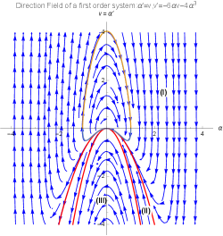
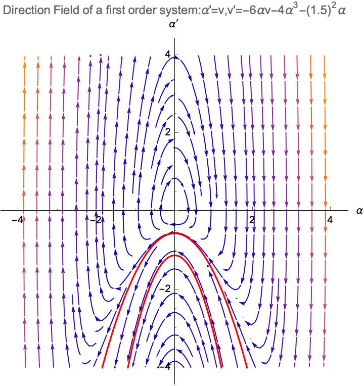
If we imagine a simple dynamical system consisting of a particle of unit mass moving on the -axis, and if is the force acting on it, then (4.31) is the equation of motion. The values of (position) and (velocity), which at each instant characterize the state of the system, are called its phases, and the plane of the variables and is called the phase plane. Using to see that (4.31) can be replaced by the equivalent system
| (4.32) |
In general, a solution of (4.32) is a pair of functions and defining a curve on the phase plane. It follows from the standard theory of ODE that if is any number and is any point in the phase plane, then there exists a unique solution of (4.32) such that and . If this solution is not a constant, then it defines a curve on the phase plane called a path of the system; otherwise, it defines a critical point. All paths together with critical points form a directed singular foliation on the phase plane with critical points as singular points of the foliation, and each path lies in a leaf of the foliation. It is easy to see that this foliation is defined by the vector field and is the only critical point. We express the direction field (or the directed singular foliation) as Figure 4.2 (Figure 4.2 for ) as follows.
5. The classification of constant -mean curvature surfaces
5.1. The classification of -minimal surfaces
Theorem 1.2 suggests we divide (locally) the -minimal surfaces into several classes. In terms of compatible coordinates , the function is a solution to the Codazzi-like equation (4.1) for any given . By Theorem 1.2, the function hence has one of the following forms of special types
and general types
where, instead of constants, both and are now functions of . Notice that for all . We now use the types of the function to define the types of -minimal surface as follows.
Definition 5.1.
Locally, we say that a -minimal surface is
-
(1)
vertical if vanishes (i.e., for all ).
-
(2)
of special type I if .
-
(3)
of special type II if .
-
(4)
of general type if with for all .
We further divide -minimal surfaces of general type into three classes as follows:
Definition 5.2.
We say that a -minimal surface of general type is
-
(1)
of type I if for all .
-
(2)
of type II if for all , and either or .
-
(3)
of type III if for all , and .
We notice that the type is invariant under an action of a Heisenberg rigid motion and the regular part of a -minimal surface is a union of these types of surfaces. The corresponding paths of each type of are marked on the phase plane (Figure 4.2). We express some basic facts about -minimal surfaces with type as follows.
-
•
If vanishes, then it is part of a vertical plane.
-
•
The two concave downward parabolas represent respectively. The one for is on top of the one for . For surfaces of special type I, we have that
(5.1) and, for surfaces of special type II, we have that
(5.2) -
•
The closed curves with the origin removed correspond to the family of solutions
where are constants and , which are of type I. There exists a zero for -function at . For surfaces of type I, we have , so is a bounded function for each fixed , that is, along each path on the phase plane, is bounded. Therefore, there are no singular points for surfaces of type I.
-
•
The curves in between the two concave downward parabolas are of type II. The -function of type II does not have any zeros. For surfaces of type II, it can be checked that
(5.3) -
•
The curves beneath the lower concave downward parabolas are of type III. There exists a zero for -function at . For surfaces of type III, we have
(5.4)
Proposition 5.3.
Suppose , which is of general type. Then the explicit formula for the induced metric on a -minimal surface with this as its -function is given by
| (5.5) |
for some functions and .
Proof.
Similarly, we have
Proposition 5.4.
Suppose , which is of special type I. Then the explicit formula for the induced metric on a -minimal surface with this as its -function is given by
| (5.6) |
Proof.
To obtain (5.6), we choose as an anti-derivative of with respect to . ∎
Proposition 5.5.
Suppose , which is of special type II. Then the explicit formula for the induced metric on a -minimal surface with this as its -function is given by
| (5.7) |
Proof.
To have (5.7), we choose as an anti-derivative of with respect to . ∎
5.2. Analogs for constant -mean curvature surfaces
If (we assume that ), then the Codazzi-like equation (1.2) has the trivial solution and the general solution of the form
| (5.8) |
which depends on two constants and .
Proposition 5.6.
For any , the explicit formula for the induced metric on a constant -mean curvature surface with as its -mean curvature and this as its -function is given by
| (5.9) |
and
| (5.10) |
for some functions and .
Proof.
Let . Then . If we choose , it is easy to see
and hence,
where
Direct computations imply
| (5.11) |
and
| (5.12) |
∎
Example 5.7 (Pansu Sphere).
The Pansu sphere in [5] is the union of graphs of and given by
which has a constant -mean curvature . Its -function is of the following form,
and the metric is given by
| (5.13) |
6. A representation of constant -mean curvature surfaces
Let be a -minimal surface. We define an orthogonal coordinate system to be a compatible coordinate system such that , that is, .
Proposition 6.1.
There always exists an orthogonal coordinate system around any regular point of a -minimal surface .
Proof.
Suppose that is a regular point and is an arbitrary compatible coordinate system around . Since , equations (2.15) and (2.18) imply that the ratio is just a function of . Now we define another compatible coordinates by
for some functions and such that . By the transformation law (2.20) of the representation of the induced metric, we have . This means that are orthogonal coordinates around . ∎
6.1. The proof of Theorem 1.3
It will be suitable to choose an orthogonal coordinate system to study a -minimal surface. One sees easily from (2.19) and (2.20) that any two orthogonal coordinate systems and are transformed by
| (6.1) |
for a constant and a function . That is, the orthogonal coordinate systems are determined, up to a constant on the coordinate and scaling on the coordinate . The transformation law of the representation of the induced metric hence reduces to
| (6.2) |
In terms of orthogonal coordinate systems, the integrability condition hence reads
| (6.3) |
Then the -function determines the metric representation , and hence a -minimal surface, up to a positive function as (2.15) specified (or see (5.5),(5.6) and (5.7) ). Therefore, from the transformation law of the induced metric (6.2), we are able to choose another orthogonal coordinate system with satisfying . That is, we can further normalize such that for each type, no matter it is special or general. Here is the function in the numerator of (see (5.5),(5.6) and (5.7)) with replaced by . In fact, for a general type (the special types are similar), it is possible to choose another orthogonal coordinate system such that
One sees that such orthogonal coordinate systems are unique up to a translation on the two variables and . In other words, there are constants and such that
| (6.4) |
We call such an orthogonal coordinate system a normal coordinate system. Indeed, since , Definition 5.1 indicates the following transformation law for and functions
| (6.5) |
where and are with respect to . Namely, is unique up to a translation on , and
is unique up to a translation on and its image as well. We denote these two unique functions and by and , respectively. We then complete the proof of Theorem 1.3.
Both two functions and are invariants under a Heisenberg rigid motion. Therefore we call them - and -invariants, respectively. In terms of and , we thus have the version of the fundamental theorem for -minimal surfaces in (Theorem 1.5).
6.2. The proof of Theorem 1.5
Given , for (1) in Theorem 1.5, we define on by
Notice that needs to be chosen so that does not contain the zero set of . Then they satisfy the integrability condition (3.1) with , and hence together with can be embedded into to be a -minimal surface with as its -function, and the induced metric . Moreover the characteristic direction . From the type of , this minimal -surface is of special type I. In view of and , we see that the coordinates are a normal coordinate system. Therefore is the corresponding -invariant. The uniqueness follows from the fundamental theorem for surfaces in or theorem 1.3. This completes the proof of (1) for the special type I. Both proofs of (1) for the special type II and of (3) are similar with chosen according to their types. For the special type II, note that needs be chosen so that does not contain the zero set of , and we define on by
For (3), we see that needs be chosen so that contains no the zero set of , and we define on by
Thus we complete the proof of Theorem 1.5.
We remark that, in terms of normal coordinates , the co-frame formula (2.3) reads
| (6.6) |
and hence the induced metric (the first fundamental form) reads
| (6.7) |
From (6.7), we see immediately that the induced metric degenerates on the singular set for surfaces of special type I. Therefore, it cannot extend smoothly through the singular set. On the other hand, this phenomenon does not happen for both special type II and general type.
6.3. The maximal -minimal surfaces and the proof of Theorem 1.6
From the proof of Theorem 1.5, it is clear to see that
-
•
for the special type I, the open rectangle in (1) of Theorem 1.5 can be extended to be either
(6.8) which depends on that is originally contained in or . Notice that the embedding might be just extended to be an immersion. Since both and are connected and simply connected, the immersion is unique, up to a Heisenberg rigid motion. We denote these two -minimal surfaces of special type I by and . From (6.7), we see that the induced metric degenerates on the singular set .
-
•
for the special type II, the open rectangle in (2) of Theorem 1.5 can be extended to be either
(6.9) which depends on the fact that is originally contained in or . The embedding might be extended to be an immersion. Since both and are connected and simply connected, the immersion is unique, up to a Heisenberg rigid motion. We denote these two -minimal surfaces of special type II by and .
-
•
when for all , since there exist no zeros of , the open rectangle in (3) can be extended to be the product space
Since the extended immersion is unique, up to a Heisenberg rigid motion, we denote the -minimal surface of type I by .
-
•
when for all , since the zero set consists of two separated curves defined by and , respectively, the open rectangle in (3) can be extended to be one of the following three domains:
(6.10) Since the extended immersion is unique, up to a Heisenberg rigid motion, we denote these two -minimal surfaces of type II by and , and the -minimal surface of type III by .
We see that -invariant is the only invariant for -minimal surfaces of special types, and - and -invariants are the only two invariants for general type. From the above, Theorem 1.6 immediately follows.
6.4. Symmetric -minimal surfaces
A -minimal surface is called symmetric if -invariant is a constant for the special types; both - and -invariants are constants for the general types. Since , up to a translation on its image, is an invariant, we presently have
Theorem 6.2.
All symmetric -minimal surfaces of the same special type are locally congruent to one another, whereas for the general type, locally there is a family of symmetric -minimal surfaces, depending on a parameter on .
6.5. The normalization of constant -mean curvature surfaces
Unlike -minimal surfaces, Proposition 5.6 indicates that normalizing to be zero is not applicable. Therefore, we would like to normalize and so that they look like the induced metric of the Pansu sphere given in (5.13) as possible as we can. Let be another compatible coordinates. The transformation laws imply
| (6.11) |
where we have the sign ”” if . Therefore, if we can choose such that , we have
| (6.12) |
Similarly,
| (6.13) |
which implies that if is chosen to be , we obtain
| (6.14) |
It is easy to see that such a coordinate system is unique up to a translation, i.e., for some constants . We call it the normal coordinate system.
Theorem 6.3.
In normal coordinates , the functions and in the expression are unique in the following sense: up to a translation on , is unique up to a sign; and is unique up to a constant. We denote these two unique functions by
Therefore, is a complete set of invariants for those surfaces ( not vanishing).
7. Examples of -minimal surfaces
7.1. Examples of special type I
The following is a family of -minimal surfaces. They are defined by the graphs of
| (7.1) |
for some real constants and . It is easy to see that or is the only singular point of the graph of .
Lemma 7.1.
The graph defined by (7.1) is congruent to the graph of .
Proof.
After the action of the left translation by , we have
This completes the proof. ∎
Example 7.2.
The p-minimal surface defined by the graph of corresponds to , where . Indeed, let us consider a surface defined by
The horizontal normal can be calculated as
| (7.2) |
and then
| (7.3) |
For the -function, making use of
to derive , and hence is the only singular point. Notice that is not a compatible coordinate system. In terms of the polar coordinates with the coordinates transformation and , that is, we consider the re-parametrization
It represents
| (7.4) |
From (7.3), it is easy to see that , and thus is a compatible coordinate system. For the -function and the induced metric and , we solve the equation
to get from (7.2), and to obtain
which, from the formula of , implies that the polar coordinates is a normal coordinate system. Since , the surface is of special type I with the as -invariant, and hence is a symmetric -minimal surface.
Given Theorem 6.2, we immediately have the following theorem.
Theorem 7.3.
A symmetric -minimal surface of special type I is locally congruent to the graph of .
Proof.
This is because that is constant for a symmetric -minimal surface of special type I and the function , up to a constant, is a complete invariant. ∎
Theorem 7.4.
In terms of normal coordinates , the induced metric (the first fundamental form) on a -minimal surface of special type I degenerates on the singular set . Therefore if it is not symmetric, then it will never smoothly extend through the singular set.
Proof.
In terms of normal coordinates, a -minimal surface of special type I is given by a function , in which we have
Therefore,
This is equivalent to that the induced metric is degenerate on the singular set on which blows up. In fact, we have
where is the dual co-frame of . If it is not symmetric, and suppose that it can be smoothly extended beyond the singular set, then the singular set is actually a singular curve and the induced metric must be non-degenerate. This completes the proof. ∎
7.2. Examples of special type II
The other family of -minimal surfaces is defined by the graph of
| (7.5) |
for some real constants and such that and .
Lemma 7.5.
The graph defined by (7.5) is congruent to the graph of .
Proof.
Since , the matrix
defines a rotation on . Let
we have
which implies
This completes the proof. ∎
Example 7.6.
We now study the example of the graph of . We consider a parametrization of the graph defined by
then we have
| (7.6) |
The horizontal normal is taken to be
where . Combining with (7.6), one sees
| (7.7) |
We proceed to compute the -function, and in terms of , which is a compatible coordinate system. These are obtained from immediately as follows.
| (7.8) |
(i) Thus, from the formula of , the coordinates is a normal coordinate system on the part where , and we have . It is easy to see that the graph of , for , is just the maximal surface when we restrict to the domain .
(ii) For the other part with , we have . Therefore, instead of , the new coordinate system is a normal coordinate system (notice that the compatible coordinates are chosen so that ). The invariants and read
| (7.9) |
and hence . Here ′ means the derivative with respect to .
(iii) For the other part with , we can say something more. If, instead of , we choose as the characteristic direction, that is, , then the coordinates lead to the normal coordinate system for the part with . As a result, we consider the re-parametrization of the surface
such that . Similarly, from , we have
| (7.10) |
where is defined by . Thus is the normal coordinate system and we have .
Let and be the part of the surface with and , respectively. In terms of the notations defined in Subsection 6.3, we see that and . Then, comparing with (7.8) and (7.10), we immediately have the following proposition, due to Theorem 1.5.
Proposition 7.7.
The surface and are congruent to each other. They in fact differ by an action of the Heisenberg rigid motion .
Theorem 7.8.
Any -minimal surface of special type II is locally a part of the surface defined by for some , up to a Heisenberg rigid motion. In addition, it is symmetric if and only if is linear in the variable . Therefore, any symmetric -minimal surface of special type II is locally a part of the surface defined by the graph of , up to a Heisenberg rigid motion.
Proof.
Any -minimal surface of special type II locally has the following normal representation
| (7.11) |
in terms of normal coordinates . Therefore, comparing with (7.8), the proof is finished if we choose such that . Moreover, it is symmetric if and only if constant, i.e., is linear in . ∎
7.3. Examples of types I, II and III
We consider the surface defined on by
| (7.12) |
Then it can be calculated that
Notice that , and , i.e., is independent of and . We rewrite as
| (7.13) |
which is a vector tangent to the contact plane. Then we choose , and hence , which yields
| (7.14) |
This implies that such surface defined by (7.12) has -mean curvature . We proceed to work out the -function , and . By definition, it is a function satisfying , that is,
| (7.15) |
for some functions . Similarly, we rewrite as a linear combination of and , and we can express as
| (7.16) |
Combining (7.15) and (7.16) and notice that , we obtain that and hence
If , then we have . However, if , then , and read
| (7.17) |
which means that is an orthogonal coordinate system, but not normal. In particular, if for all , then one sees that the -minimal surface has no singularities. From (7.17), we conclude that
this surface is of type I if for all . On the other hand, if for all , then it is either of
type II on which or ; or type III on which .
Finally, we can further take the coordinates to normalize such that it only depends on and , then we have
| (7.18) |
for some constant , and hence
| (7.19) |
8. Structures of singular sets of -minimal surfaces
In this section, we assume that is a -minimal surface.
Proposition 8.1.
Let be a singular point of a -minimal surface . Then there must be a characteristic line approaching this point .
Proof.
Suppose no characteristic line approaches this point . We would like to find a contradiction. Firstly, by [3], there exists a small neighborhood of whose intersection with the singular set is contained in a smooth curve . If the neighborhood is small enough, then, on one side of the curve , we can find a compatible coordinate system such that is contained on the boundary of . Notice that, by our assumption, does not lie at the end of any leaf of the foliation defined by . Thus the image of the map defined on by is bounded on the phase plane (see Figure 4.2). Therefore, we have that is finite, which is a contradiction since is a singular point. ∎
8.1. The proof of Theorem 1.7
Due to Proposition 8.1, it suffices to show this theorem for a -minimal surface of some type. For general type (notice that there are no singular points for type I), we choose a normal coordinate system such that , and read
| (8.1) |
where is a positive function of the variable such that . Then the singular set is the graphs of the functions
| (8.2) |
By (6.7), the induced metric (or the first fundamental form) on the regular part reads
| (8.3) |
Now we use the metric to compute the length of the singular set , where belongs to some open interval. Let , which is a parametrization of the singular set. Then the square of the velocity at is
| (8.4) |
where we have used the fact that on the singular set. Formula (8.4) shows that the parametrized curve of the singular set has a positive length. We omit similar proof for special type II.
Finally, for special type I, in terms of a normal coordinate system , we have
| (8.5) |
If is a parametrization of the singular set for inside some open interval, then (6.7) indicates that the induced metric on the regular part reads
| (8.6) |
and the square of the velocity at is
| (8.7) |
where we have used the fact that on the singular set. From formula (8.7), we see that the length of depends on whether the value is zero or not, which implies that the singular set is either an isolated point or a smooth curve of positive length. In addition, the singular set as an isolated point happens if and only if is a constant, that is, the surface is part of a plane. We thus complete the proof of this theorem 1.7.
8.2. The proof of Theorem 1.8
Around the singular point , we may assume that the surface is represented by a graph . Let be a parametrization of the -minimal surface around defined by . Then
| (8.8) |
which yields
where is the induced metric (first fundamental form) on the surface. Now we choose a horizontal normal as follows
where . Then
| (8.9) |
is tangent to the characteristic curves.
We first claim that either or . Let and let be a parametrization of the singular curve passing through . Notice that we may assume, w.l.o.g., that the -axis past is transverse to the singular curve, i.e., . Since , taking derivative with respect to gives . Therefore, if , and hence .
If , we turn to compute the angle between and . First, from (8.8), we have
On the other hand, using (8.9) to get
Combining the above two formulae, we obtain
| (8.10) |
where the sign depends on that the sign of is positive or not. By the mean value theorem, it is easy to see (or see [3]) that
| (8.11) |
and thus
| (8.12) |
where means that from the side in which is positive (negative).
If , similar computations give the angle between and by
| (8.13) |
thus
| (8.14) |
where means that from the side in which is positive (negative).
From (8.11), it is easy to see that both and differ by a sign on the different side of the singular curve which is defined by and . Therefore, from the formula of (see (8.9)), together with (8.12) and (8.14), we conclude that the characteristic vector field differs by a sign on the different side of the singular curve when approaching the singular point . This completes the proof of theorem 1.8.
8.3. The proof of Theorem 1.9
In terms of normal coordinates , the surface is represented by two functions and . Since it is of type II, we have and
| (8.15) |
on which either or . The induced metric is
| (8.16) |
We assume that lies on the part (the proof for the case that lies on the part is similar). Suppose, in addition, that can be smoothly extended beyond the singular curve . By theorem 1.8, the coordinates can be extended beyond the singular curve to be compatible coordinates. Then the -function on the other side of the singular curve must be one of the following
-
(1)
, which is of special type I;
-
(2)
, which is of special type II;
-
(3)
, which is of general type,
for . The induced metric on this other part is
| (8.17) |
Comparing (8.16) and (8.17), and noting that is smooth around the singular curve, we have
with . That is, cases (1) and (2) for do not happen. Therefore, the extended coordinates beyond the singular curve are also normal coordinates. The formula of shows that the part on the other side of the singular curve is of type III. This completes the proof of Theorem 1.9.
8.4. The proof of the Bernstein-type theorem
In this subsection, we will show that (7.1) and (7.5) are the only entire smooth -minimal graphs. Suppose that is an entire -minimal graph. First of all, since it is a graph, we notice that there is nowhere at which is zero. Next, we claim the following lemma.
Lemma 8.2.
The induced singular characteristic foliation of does not contain a leaf along which is of general type, that is, in terms of normal coordinates around the leaf, is a general solution of the Codazzi-like equation see (4.1).
Proof.
Suppose not. We assume that the induced singular characteristic foliation of contains such a leaf. Then there will be a piece of the surface (a neighborhood) around the leaf such that this piece is of general type. Suppose that this piece is of type I or of type III, then the entireness and the phase plane (Figure 4.2) indicate that the -function must be extended so that it has a zero somewhere. This is a contradiction. Therefore this piece (of general type) must be of type II. Again, since it is entire, this piece can be smoothly extended through the singular curve. By Theorem 1.9, it contains a piece of type III, which lies on the other side of the singular curve. This is also a contradiction, as we argue above. We hence complete the proof of Lemma 8.2. ∎
From Lemma 8.2, we know that an entire -minimal graph is either of special type I or of special type II. If it is of special type II, Theorem 7.8 and Lemma 7.5 ensure that is one of the graphs in (7.5). If it contains a piece of special type I, then this piece must be symmetric by Theorem 7.4. Therefore, by Theorem 7.3 and Lemma 7.1, the surface must be one of the graphs in (7.1). We hence complete the proof of the Bernstein-type theorem. We also remark that the Bernstein-type theorem still holds for surfaces in .
Remark 8.3.
We point out that in [3], the Bernstein-type theorem had been proved in -graphs.
9. An approach to construct -minimal surfaces
In this section, we provide an approach to constructing -minimal surfaces. It turns out that, in some sense, generic -minimal surfaces can be constructed by this approach, particularly, other than those -minimal surfaces of special type I. This approach is to perturb the surface in some way. Recall we choose the parametrization of by
where each half-ray with a fixed angle is a Legendrian straight line. Therefore, the image of the action of each Heisenberg rigid motion on is also a Legendrian straight line. Let be an arbitrary curve . Then for each fixed and , the curve defined by
is a Legendrian straight line. Here is the left translation by . Therefore, the union of these lines constitutes a -minimal surface with a parametrization given by
| (9.1) |
This surface depends on the curve . We have the following proposition about the surface .
Proposition 9.1.
The coordinates are compatible coordinates for . In terms of this coordinate system, the -invariant and the induced metric read
| (9.2) |
and
| (9.3) |
where .
Proof.
We make a straightforward computation for the invariants and . Firstly, we have
| (9.4) |
From the construction of , we have . Thus
| (9.5) |
whereas we have
If we let
| (9.6) |
for some functions and . Then straightforward computations show that
| (9.7) |
We recall that the three invariants and are related by
| (9.8) |
If we substitute (9.4), (9.5) and (9.6) into (9.8), and compare the corresponding coefficients, we then obtain (9.2) and (9.3). ∎
We conclude that is an immersion if and only if either for all , where .
Formula (9.3) suggests the following: That defines a -minimal surface of special type depends on whether vanishes or not.
Comparing equations (1.12) and (1.14), it is convenient to regard surfaces of special type I as surfaces of general type with -invariant vanishing. Now given two arbitrary functions and , we solve equation system (1.14) for a smooth curve . Since system (1.14) is equivalent to the following system
| (9.9) |
which is underdetermined. Therefore, the solutions always exist. For example, we can solve the first equation of (9.9) for and then solve for from the second one. It turns out that we can find a smooth curve such that the corresponding -minimal surface has the two given functions and as its -and -invariants. If , then is of special type I. We thus conclude, together with Theorem 7.8 in which states parametrizations for -minimal surfaces of special type II, that we generically have provided a parametrization for any given -minimal surface with type. In particular, we give a parametrization presentation for the eight classes of maximal -minimal surfaces constructed in Subsection 6.3.
Finally, we point out that these -minimal surfaces constructed by curves defined by (1.10) and (1.13) are all immersed surfaces at least (in some cases, they are embedded). This is because that for all points. In particular, formula (1.14) says that if then
which is not zero.
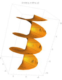
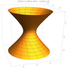
Example 9.3.
Example 9.4.
If we take to be the curve , then
The surface of type I in Subsection LABEL:exat1 (see Figure 7.4) can be recovered by taking a rotation by about the -axis.
References
- [1] V. Barone Adesi, F. Serra Cassano, and D. Vittone, The Bernstein problem for intrinsic graphs in Heisenberg groups and calibrations, Preprint.
- [2] T. A. Burton, The Nonlinear Wave Equation as a Liénard Equation, Funkcialaj Ekvacioj, 34 (1991) 529-545.
- [3] Cheng, J.-H.; Hwang, J.-F.; Malchiodi, A., and Yang, P., Minimal surfaces in Pseudohermitian geometry, Annali della Scuola Normale Superiore di Pisa Classe di Scienze V , 4 (1), 129-177, 2005.
- [4] Cheng, J.-H.; Hwang, J.-F.; Malchiodi, A., and Yang, P., A Codazzi-like equation and the singular set for smooth surfaces in the Heisenberg group, J. Reine angew. Math. 671 (2012), 131-198.
- [5] Cheng, J.-H.; Chiu, H.-L.; Hwang, J.-F., and Yang, P.,Umbilicity and characterization of Pansu spheres in the Heisenberg group, Journal fur die reine und angewandte Mathematik (738), 203-235, 2018.
- [6] Chiu, H.-L. and Lai, S.-H., The fundamental theorem for hypersurfaces in Heisenberg groups, Calc. Var. Partial Diffrential Equations, 54 (2015), no. 1, 1091-1118.
- [7] D. Daniekki, N. Garofalo, D. M. Nhieu and S. D. Pauls, Instability of graphical strips and a positive answer to the Bernstein problem in the Heisenberg group , J. Differential Geometry, 81, pp 251–295, 2009.
- [8] D. Danielli, N. Garofalo, DM Nhieu and S., Pauls, The Bernstein problem for Embedded surfaces in the Heisenberg group , Indiana University mathematics journal, pp 563-594, 2010.
- [9] Zaitsev, V. F. and Polyanin, A. D., Discrete-Group Methods for Integrating Equations of Nonlinear Mechanics, CRC Press, Boca Raton, 1994.
- [10] Polyanin, A.D. and Zaitsev,V.F., Handbook of Exact Solutions for Ordinary Differential Equations, 2nd Edition, Chapman and Hall/CRC, Boca Raton, 2003.
- [11] Liénard, A., Etude des oscillations entretenues, Revue Générale de l’Electricité 23 (1928) 901-912 & 946-954.
- [12] A. Chiellini, Sull’integrazione dell’equazione differenziale , Bollettino dell’Unione Matematica Italiana, 10, 301-307 (1931).
- [13] M. J. Ablowitz, D. J. Kaup, A. C. Newell and H. Segur, Method for solving the Sine-Gordon equation, Phy. Rev. Lett. 30 (1973),1262–1264
- [14] M. Remoissenet, Waves Called Solitons: Concepts and Experiments, Springer, 1994.
- [15] A. Bäcklund, Zur Theorie der Flächentransformationen, Math. Ann. XIX 387–422 (1882).
- [16] A. Bäcklund, On ytor med konstant negativ krökning, Lunds Univ. rsskr XIX (1883).
- [17] A. Bäcklund, Einiges über Kugelkomplexe, Annali di Matematica Ser III XX 65–107 (1913).
- [18] O. Calin, Geodesics on a certain step 2 sub-Riemannian manifold, Number 22. Annals of Global Analysis and Geometry, pp. 317-339, 2002.
- [19] O. Calin, D. C. Chang, and P. C. Greiner, On a Step 2(k + 1) sub-Riemannian manifold, volume 14. Journal of Geometric Analysis, pp. 1-18, 2004.
- [20] U. Hamenstiidt, Some regularity theorems for Carnot-Caratheodory metrics, volume 32. J. Differential Geom., pp. 819-850, 1990.
- [21] P. Hartman, Ordinary Differential equations, Wiley, 1984.
- [22] W. Liu and H. J. Sussmann, Shortest paths for sub-Riemannian metrics on rank two distri- butions, volume 118. Mem. Amer. Math. Soc., 1995.
- [23] R. Beals, B. Gaveau, and P. C. Greiner, Hamilton-Jacobi theory and the heat kernel on Heisenberg groups, Number 79. J. Math. Pure Appl., pp. 633-689, 2000.
- [24] R. Beals, B. Gaveau, and P.C. Greiner, On a Geometric Formula for the Fundamental Solu- tion of Subelliptic Laplacians, Number 181. Math. Nachr., pp. 81-163, 1996.
- [25] O. Calin, D. C. Chang, and P. C. Greiner, Geometric mechanics on the Heisenberg group, Bulletin of the Institute of Mathematics, Academia Sinica, 2005.
- [26] O. Calin and V. Mangione, Variational calculus on sub-Riemannian manifolds, volume 8, Balcan Journal of Geometry and Applications, 2003.
- [27] B. Gaveau, Principe de moindre action, propagation de la chaleur et estimees sous-elliptiques sur certains groupes nilpotents, volume 139. Acta Math, 1977, pp. 95-153.
- [28] A. Koranyi, Geometric properties of Heisenberg groups, Advances in Math., pp. 28-38, 1985.
- [29] A. Koranyi, Geometric aspects of analysis on the Heisenberg group, Topics in Modern Harmonic Analysis, pp. 209-258, May-June 1982.
- [30] A. Koranyi and H. M. Riemann, Quasiconformal mappings in the Heisenberg group, Invent. Math., pp. 309-338, 1985.
- [31] Gerald B. Folland, Fourier Analysis and its Applications, Brooks / Cole, Pacific Grove, 1992.
- [32] Karl-Heinz Gröchenig, Foundations of Time-Frequency Analysis, Birkhäuser, Boston, 2000.
- [33] Ernst Binz and Sonja Pods, The Geometry of Heisenberg Groups With Applications in Signal Theory, Optics, Quantization, and Field Quantization, AMS 2008.
- [34] Malchiodi, A., Minimal surfaces in three dimensional pseudo-Hermitian geometry, Lecture Notes of Seminario Interdisciplinare di Matematica, Vol. 6, pp. 195-207, 2007.
- [35] S. D. Pauls, Minimal surfaces in the Heisenberg group, Geometriae Dedicata,104, pp. 201-231, 2004.
- [36] M. Ritoré and C. Rosales, Rotationally invariant Hypersurfaces with constant mean curvature in the Heisenberg group , The Journal of Geometric Analysis, v.16, n.4 pp. 703-720 (2006).