A Central Difference Graph Convolutional Operator for Skeleton-Based Action Recognition
Abstract
This paper proposes a new graph convolutional operator called central difference graph convolution (CDGC) for skeleton based action recognition. It is not only able to aggregate node information like a vanilla graph convolutional operation but also gradient information. Without introducing any additional parameters, CDGC can replace vanilla graph convolution in any existing Graph Convolutional Networks (GCNs). In addition, an accelerated version of the CDGC is developed which greatly improves the speed of training. Experiments on two popular large-scale datasets NTU RGB+D 60 & 120 have demonstrated the efficacy of the proposed CDGC. Code is available at https://github.com/iesymiao/CD-GCN.
Index Terms:
Graph Convolutional Network, Action Recognition, Skeleton.I Introduction
Human action recognition is a pupular and challenging research topic. It has attracted extensive attention in different research fields in recent years [1, 2, 3, 4, 5] due to its wide range of applications such as video analytic, robotics, human-machine interactions and health and aged care. Skeleton is one of the effective representations of human motion. It is not only robust against interference from background but also has computational advantages, as each skeleton consists of a small number of joints. Therefore, much recent research is based on 3D skeletons [6, 7, 8, 9, 10, 11, 12, 13].
Among the reported approaches to skeleton based action recognition, graph convolutional network (GCN) has shown much more promising performance than convolutional neural network (CNN) and/or recurrent neural network (RNN) based approaches [14, 15, 16, 9, 13], mainly due to the fact that a skeleton can be naturally considered as a graph where each joint being a node and an anatomic link between two joints being an edge in the graph. To date, many GCN-based methods take joint locations or coordinates directly as input of their models. In [17], bones calculated from adjacent and anatomically connected joints are introduced as an additional input modality for the first time, leading to an improvement of the recognition performance. However, both joints and bones are defined by body’s anatomic structure. On one hand, extensive research has been conducted on improving the topology of a skeleton graph by including dynamic links between joints. For example, 2s-AGCN [17] employs additional non-local neural network modules to learn an effective graph topology. AS-GCN [14] proposes an encoder-decoder structure to capture action-specific links. On the other hand, many works adopting GCN attempt to extract richer features by either expanding the space-time perception domain [18] or devising complex multi-stream network architectures [19, 20]. However, these methods directly use vanilla graph convolution operations to aggregate information from the associated nodes in the graph topology for the central node, ignoring the local motion information between the central node and the neighboring nodes, as shown in Fig. 1(a).
Our hypothesis is that improving the graph convolution operator itself via incorporating the local motion information among the nodes could be as effective as improving the topology of a skeleton graph. To this end, this letter proposes a novel graph convolution operator called Central Difference Graph Convolution (CDGC) for skeleton based action recognition. It can capture the dynamic gradient information related to the local motion between the central node and its associated neighboring nodes during feature aggregation, as shown in Fig. 1(b). Besides, the proposed CDGC does not introduce any additional parameters and it can be used to replace vanilla graph convolution in any existing graph convolution neural networks to improve their performance. In addition, an accelerated version of CDGC is developed, which greatly improves the training speed of the network. Extensive experiments on two large-scale benchmark datasets have demonstrated the efficacy of the proposed CDGC.

II Proposed Method
This section first gives an overview of the Vanilla Graph Convolution in Sec. II-A. The proposed Central Difference Graph Convolution (CDGC) and its implementation are detailed in Sec. II-B and II-C, respectively. Its accelerated version is presented in Sec. II-D.
II-A Vanilla Graph Convolution
A graph is usually represented as , where is a set of nodes representing joints of a skeleton and is a set of edges representing bones between joints. Given a skeleton graph, multiple layers of vanilla graph convolutions are applied to extract multi-level features. Suppose is a vertex in the graph, a vanilla graph convolution operation centred at it is expressed as:
| (1) |
where x and y denote an input feature map and output feature map, respectively. w is the weight function that provides a weight vector based on the given input. is the 1-distance neighboring vertexes of . is a partitioning function to partition vertexes in into a fixed number of subsets, with each subset having its own convolution weight vectors. In the classic partition strategy [15], is divided into three subsets: , , and . In specific, is itself; is the centripetal subset which contains vertexes closer to skeleton gravity center in ; and is the centrifugal subset which contains vertexes away from skeleton gravity center. denotes a normalizing term which balances the contribution of each subset to the output.
In general, there are two main steps in the vanilla graph convolution: 1) sampling neighboring vertexes of over the input feature map x; and 2) aggregating the values of neighboring vertexes and itself via weighted summation.
II-B Central Difference Graph Convolution
Central difference convolution (CDC) introduces the central-oriented local gradient features to enhance model’s discrimination capacity, which has been applied in many fields, such as face anti-spoofing[21, 22, 23, 24], remote heart rate measurement[25] and gesture recognition[26], and has achieved great results. Inspired by the CDC networks, we propose to integrate spatial gradient information into the graph convolution operator to enhance its representation and generalization capability.
The proposed central difference graph convolution also consists of two steps, i.e., sampling and aggregation. The sampling step is similar to vanilla graph convolution while the aggregation step is different. As shown in Fig. 1(a), central difference graph convolution prefers to aggregate the center-oriented gradient of sampled vertexes, which is expressed as:
| (2) |
When , the gradient value is always equal to zero relative to the central location itself.
For action recognition, existing works focus on establishing dynamic or action specific connections between nodes, so as to aggregate information from either explicitly or implicitly associated nodes. However, the gradient between connected nodes is also potentially useful according to the work of CDC [21]. Hence, the combination of vanilla graph convolution and central difference graph convolution is expected to provide robust and differentiated modeling capability. Thus, the above-mentioned central difference graph convolution is generalized to:
| (3) | ||||
where hyperparameter tradeoffs the contribution between nodes and gradient information. Eq.(3) is referred to as central difference graph convolution (CDGC).

Notice that the gradient information in CDGC is different from that carried by the commonly used bone modality. First, each bone points from its source joint to the target joint. The source joint is defined as the closer one to the center of gravity of skeleton, and the target joint is defined as the further one. Thus, the direction of each bone is fixed, as shown in Fig. 2(a). However, in CDGC, when one of two adjacent nodes is taken as the center node, the direction of the gradient vector is opposite to that obtained when the other node is taken as the center node. According to Eq.(2) and as shown in Fig. 2(b), when is the center, the gradient direction of relative to points from to . When is the center, the gradient direction of relative to points from to , which is opposite to the former. Thus, the information they captured is different. Second, when a connection is established between two nodes that are not connected in the nature skeleton graph, the difference between them is more prominent. If there is a coordination between hand and feet in an action, the gradient information of will be captured by the proposed CDGC when calculating the feature of . However, there is no bone between the two nodes.
II-C Implementation
A vanilla graph convolution is implemented [15] as:
| (4) |
Here the weight vectors of multiple output channels are stacked to form the weight matrix W. A is a normalized adjacency matrix. In order to simplify the expression of the subsequent formula, we omit the non-linear activation function here. In practice, the input feature map is represented as a tensor of dimensions, where and denote the number of channels, frames, and vertexes, respectively. The graph convolution is implemented by multiplying the input feature map with the normalized adjacency matrix A on the second dimension and then performing a standard 2D convolution.
Eq.(2) can be rewritten to:
| (5) | ||||
In implementation, the summation of trainable parameters in front of can be obtained by summing the second dimension of the adjacency matrix. Therefore, the implementation of the central difference graph convolution can be expressed as:
| (6) |
where is obtained by first summing the second dimension of the adjacency matrix A, i.e. , and then broadcasting the resulting vector to matrix with , with 1 being the vector of dimensionality. represents the element-wise Hadamard product. Therefore, the implementation of CDGC is formulated as:
| Y | (7) | |||
II-D Accelerated Version of CDGC
In general, implementation of graph convolution depends on an adjacency matrix. The adjacency matrix represents explicit and implicit connections between nodes, then features of the connected nodes are aggregated. However, the GCNs based on an adjacency matrix is usually computationally expensive, and the calculation process is complex and time-consuming. Recently, an advanced graph convolution model called shift-GCN[16] is proposed. It utilizes a simple graph shift operation and point-wise convolutions to aggregate neighboring node features instead of regular graph convolutions. This greatly speeds up the training process of GCN. Our accelerated version of CDGC is also based on shift operations, and therefore is also computationally efficient. Moreover, the spatial shift operation makes the receptive field of each node cover the full skeleton graph, and the features of a node after shifting are composed of the features of all other nodes in the graph. Derived from this, we propose a simple solution to realize our CDGC: making difference between the original features and the shifted features.

In Fig.3, we take a single node (right hand) as an example and draw its original feature vector and shifted feature vector. Assuming that represents the feature of channel of node . represents the feature of channel of node after shift, which is from one of the channels of node . Performing obtains the gradient feature of channel for node relative to . By subtracting the original features from the shifted features, the gradient features including all body nodes relative to right hand are obtained. In general, given a spatial skeleton feature map , where stands for the number of joints in skeleton graph, and is the number of channels of each node. represents the feature map of the shifted spatial skeleton. Performing can obtain the gradient features of all the remaining nodes in the skeleton graph with respect to their central nodes.
In addition, in the accelerated CDGC, the connection strength between different nodes is the same. But the importance of human skeletons is different. Therefore, we introduce a learnable mask M and multiply it with the obtained feature map to adjust the importance of different connections. The accelerated CDGC can be expressed as:
| (8) |
where W is the weight matrix composed of weight vectors of multiple output channels. As described in Sec. II-B, both node information captured by vanilla graph convolution and gradient information extracted by CDGC are useful for recognition. Hence, we combine the ordinary shift graph convolution with the accelerated CDGC to construct an effective graph convolution operator. This operator can be expressed as:
| Y | (9) | |||
where controls the accelerated CDGC term. The higher value of is, the more important of central difference gradient information is. The accelerated CDGC is implemented according to Eq.(9).
III Experiments
The proposed CDGC is evaluated on two popular large-scale skeleton datasets, i.e., NTU RGB+D 60[29] and NTU RGB+D 120[30]. Results are compared with the state-of-the-art methods.
III-A Datasets and Evaluation Metrics
NTU RGB+D 60[29] is currently the most widely used indoor-captured action recognition dataset, which contains a total of 56,880 3D skeleton video clips. The clips are captured from three cameras with different settings. All video clips contain a total of 60 human action classes including both single-actor and two-actor actions. Original work[29] suggests two evaluation protocols: Cross-Subject (CS) and the Cross-View (CV). In the CS evaluation, the dataset is divided into training and testing sets according to the subjects. The training set contains 40,320 videos from 20 subjects, and the rest 20 subjects with 16,560 video clips are used for testing. In the CV evaluation, dataset is divided by the camera ID number. The 37,920 videos captured from camera two and three are used in the training and the 18,960 videos from camera one are used for testing. We report the Top-1 accuracy on both protocols. For inputs with more than one stream, e.g., bones, a score-level fusion result is reported.
NTU RGB+D 120[30] is more challenging since it involves more subjects and action categories. The dataset contains 114,480 action samples in 120 action classes. Samples are captured by 106 volunteers with three cameras views. This dataset contains 32 setups, and each setup denotes a specific location and background. According to[30], this dataset suggests two evaluation metrics: Cross-Subject and Cross-Setup. The former one splits subjects in half to training and testing parts while the latter one divides the samples based on the camera setup IDs.
III-B Experimental Settings
Our model is based on shift-GCN. Specifically, the model consists of one input block and nine basic blocks. In each basic block, we use the proposed accelerated CDGC to learn spatial features, and the temporal correlation is still modeled by temporal shift graph convolution. Both of them followed by a batch normalization (BN) layer and a ReLU layer. A residual connection is added to each basic block to avoid the degradation problem with the increase of network depth, and make the network easy to optimize and fast to converge. A BN layer is added at the beginning to normalize the input graph, and a global average pooling layer is added at the end to pool the feature maps of different samples into the same size. Finally, the output feature is sent to a SoftMax classifier to generate the prediction for action recognition.
All experiments are conducted on the PyTorch deep learning framework [27]. SGD with Nesterov momentum (0.9) is used to train the model for 140 epochs. Learning rate is set to 0.1 and divided by 10 at epoch 60, 80 and 100. Cross-entropy is selected as the loss function to back-propagate gradients. For NTU RGB+D 60 and NTU RGB+D 120, the batch size is 48, and we adopt the same data preprocessing as in [17]. The experiments are performed on two NVIDIA TitanXP GPU.

III-C Ablation Study
In this section, we use 2s-AGCN [17] as the backbone to evaluate the effectiveness of our method. All ablation studies are conducted on the NTU RGB+D 60 dataset.
III-C1 Impact of in CDGC
In these experiments, we use joint data as input and follow the cross-view and cross-subject protocols, respectively. According to Eq.(3), controls the contribution of the spatial gradient cues, i.e., the higher , the more gradient information are included. For the cross-view protocol, as shown in Fig.4(a), when 0 0.6, the performance of CDGC is better than vanilla graph convolution ( = 0, Accuracy = 93.82), indicating that the gradient information captured by CDGC improves recognition. The best performance is obtained when = 0.3 (Accuracy = 94.17). In the cross-subject protocol, as shown in Fig.4(b), the best accuracy is also obtained at = 0.3 (Accuracy = 86.87). Thus, we use this optimal value ( = 0.3) in the following experiments.
III-C2 Impact of CDGC
In order to verify the capability of CDGC, we replace the spatial GCN module in 2s-AGCN with the CDGC to test whether the performance will drop or increase.
| data | X-sub | X-view | |
|---|---|---|---|
| 2s-AGCN | Joint | 86.3 | 93.8 |
| 2s-AGCN(CDGC) | Joint | 86.9 | 94.2 |
| 2s-AGCN | Bone | 87.0 | 93.2 |
| 2s-AGCN(CDGC) | Bone | 87.5 | 93.9 |
| 2s-AGCN | 2s | 88.5 | 95.1 |
| 2s-AGCN(CDGC) | 2s | 89.1 | 95.5 |

The results are shown in Table I. The recognition results of the 2s-AGCN model are run by ourselves. As seen, under the cross-subject evaluation, the accuracy is improved by 0.6 and 0.5 percentage points on the joint stream and bone stream, respectively. After fusion of them, the recognition performance is improved by 0.6 percentage points. Under the cross-view evaluation, we improve the accuracy by 0.4 and 0.7 percentage points on the joint stream and bone stream, respectively. After fusion, the recognition accuracy is improved by 0.4 percentage points. Also, Fig.5 shows the accuracy comparison of each action class between 2s-AGCN and CDGC. It can be seen that the recognition accuracy of our CDGC in categories ”writing”, ”take off a shoe” and ”nod head/bow” is significantly higher than that of the baseline. For the three classes, the motion directions of the related collaborative joints and the relative motion relationship among them are important. The CDGC can not only aggregate features of neighboring nodes, but also capture the differential gradient information among them, which can reflect the motion direction and amplitude of adjacent nodes, so as to improve recognition. In addition, it should be noted that CDGC does not increase the number of parameters, but it has performance advantage over the vanilla graph convolution.
III-C3 Impact of accelerated CDGC on network training
| Time Consumption | Params | Convergence | |
|---|---|---|---|
| CDGC | 53min | 3.47M | 30th epoch |
| Accelerated CDGC | 10min | 0.69M | 60th epoch |
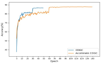
In order to verify the contribution of accelerated CDGC to the network training compared to the ordinary CDGC in Sec.II-B. We compare the two in three aspects: time consumption per epoch, model parameters and number of epochs to converge. As shown in Table II, the accelerated CDGC is significantly better than the ordinary one in the first two items as expected. Fig. 6 shows the training accuracy. We can see that CDGC converges faster and needs less number of training epochs than the accelerated CDGC. Table III compares the recognition accuracy of the two versions of CDGC. It can be seen that the recognition accuracy of the accelerated CDGC is higher than the original one for all the stream settings. This is mainly attributed to that the accelerated CDGC makes the receptive field of each node cover all the nodes in the skeleton graph.
| NTU RGB+D 60 | X-sub | X-view | ||||
| Joint | Bone | 2s | Joint | Bone | 2s | |
| CDGC | 86.9 | 87.5 | 89.1 | 94.2 | 93.9 | 95.5 |
| Accelerated CDGC | 88.0 | 88.1 | 89.7 | 94.8 | 95.0 | 95.9 |
III-D Comparison with the state-of-the-art methods
In this experiment, we combine the accelerated CDGC with shift-GCN and compare it with the state-of-the-art methods on NTU RGB+D 60 and NTU RGB+D 120. In addition, as the key hyperparameter of CDGC, in each layer of the network can also be learned together with the network training. Thus, we also conduct experimental exploration with the learnable using the same experimental settings as the chosen optimal value 0.3. Like [16], we build four stream networks: joint stream, bone stream, joint motion stream and bone motion stream. For comparison, we report the results of single-stream(joint stream), double-stream(joint stream and bone stream) and four-stream(all). In the Tables IV and V, we abbreviate them as 1s, 2s and 4s, respectively.
| methods | X-sub | X-view |
|---|---|---|
| TCN[31] | 74.3 | 83.1 |
| VA-LSTM[32] | 79.2 | 87.7 |
| ST-GCN[15] | 81.5 | 88.3 |
| DPRL[33] | 83.5 | 89.8 |
| SR-TSL[34] | 84.8 | 92.4 |
| STGR-GCN[35] | 86.9 | 92.3 |
| GR-GCN[36] | 87.5 | 94.3 |
| SAR-NAS[37] | 86.4 | 94.3 |
| 2s AS-GCN[14] | 86.8 | 94.2 |
| 2s-AGCN[17] | 88.5 | 95.1 |
| 4s Directed-GNN[38] | 89.9 | 96.1 |
| 1s Shift-GCN[16] | 87.8 | 95.1 |
| 2s Shift-GCN[16] | 89.7 | 96.0 |
| 4s Shift-GCN[16] | 90.7 | 96.5 |
| ours(=0.3 1s) | 88.0 | 94.8 |
| ours(=0.3 2s) | 89.7 | 95.9 |
| ours(=0.3 4s) | 91.0 | 96.4 |
| ours(learnable 1s) | 88.0 | 94.9 |
| ours(learnable 2s) | 89.7 | 95.8 |
| ours(learnable 4s) | 90.9 | 96.5 |
| methods | X-sub | X-setup |
|---|---|---|
| Dynamic Skeleton[39] | 50.8 | 54.7 |
| FSNet[40] | 59.9 | 62.4 |
| MT-CNN-RotClips[41] | 62.2 | 61.8 |
| Pose Evolution Map[42] | 64.6 | 66.9 |
| ST-GCN[15] | 72.4 | 71.3 |
| AS-GCN[14] | 77.7 | 78.9 |
| 1s Shift-GCN[16] | 80.9 | 83.2 |
| 2s Shift-GCN[16] | 85.3 | 86.6 |
| 4s Shift-GCN[16] | 85.9 | 87.6 |
| ours(=0.3 1s) | 81.3 | 83.2 |
| ours(=0.3 2s) | 85.0 | 86.7 |
| ours(=0.3 4s) | 86.3 | 87.8 |
| ours(learnable 1s) | 81.1 | 83.3 |
| ours(learnable 2s) | 85.0 | 86.7 |
| ours(learnable 4s) | 86.3 | 87.8 |
The bold numbers indicate that our method has improved the accuracy of skeleton-based action recognition compared with the corresponding baseline. It can be seen from Table IV that our model achieves the best performance for the cross-subject protocol, i.e. 91.0, 0.3 percentage points higher than the baseline shift-GCN with optimal value = 0.3. NTU RGB+D 120 dataset is more challenging than NTU RGB+D 60. We can see from Table V that the performance of our model is 0.4 and 0.2 percentage points higher than the baseline for both cross-subject and cross-setup protocols, respectively, and has achieved the best results among the reported to date. We can also see from the two tables that the accuracy of learnable is almost the same as that of = 0.3, which proves that = 0.3 is an optimal choice. Note that the number of parameters in our model is equal to the baseline. The results have demonstrated the effectiveness of CDGC.
IV Conclusion
In this paper, we propose a new graph convolution operator called CDGC, which not only aggregates node information as a vanilla graph convolution operation does but also aggregates gradient information between nodes. Without introducing any additional parameters, CDGC can replace vanilla graph convolution in any existing GCNs. In addition, we have developed an accelerated version of CDGC that greatly improves the training speed of the network. Experiments on two popular large-scale datasets, NTU RGB+D 60 and NTU RGB+D 120, have demonstrated the efficacy of the proposed CDGC. Importantly, the results have verified our hypothesis that improving the graph convolution operator itself could be as effective as improving the topology of a skeleton graph.
References
- [1] O. P. Popoola and K. Wang, “Video-based abnormal human behavior recognition—a review,” IEEE Transactions on Systems, Man, and Cybernetics, Part C (Applications and Reviews), vol. 42, no. 6, pp. 865–878, 2012.
- [2] M. Ramanathan, W.-Y. Yau, and E. K. Teoh, “Human action recognition with video data: research and evaluation challenges,” IEEE Transactions on Human-Machine Systems, vol. 44, no. 5, pp. 650–663, 2014.
- [3] P. Wang, W. Li, P. Ogunbona, J. Wan, and S. Escalera, “Rgb-d-based human motion recognition with deep learning: A survey,” Computer Vision and Image Understanding, vol. 171, pp. 118–139, 2018.
- [4] J. Zhang, W. Li, P. O. Ogunbona, P. Wang, and C. Tang, “Rgb-d-based action recognition datasets: A survey,” Pattern Recognition, vol. 60, pp. 86–105, 2016.
- [5] Y. Ji, Y. Yang, F. Shen, H. T. Shen, and X. Li, “A survey of human action analysis in hri applications,” IEEE Transactions on Circuits and Systems for Video Technology, vol. 30, no. 7, pp. 2114–2128, 2019.
- [6] P. Wang, Z. Li, Y. Hou, and W. Li, “Action recognition based on joint trajectory maps using convolutional neural networks,” in Proceedings of the 24th ACM international conference on Multimedia, 2016, pp. 102–106.
- [7] Y. Hou, Z. Li, P. Wang, and W. Li, “Skeleton optical spectra-based action recognition using convolutional neural networks,” IEEE Transactions on Circuits and Systems for Video Technology, vol. 28, no. 3, pp. 807–811, 2016.
- [8] C. Li, Y. Hou, P. Wang, and W. Li, “Joint distance maps based action recognition with convolutional neural networks,” IEEE Signal Processing Letters, vol. 24, no. 5, pp. 624–628, 2017.
- [9] C. Cao, C. Lan, Y. Zhang, W. Zeng, H. Lu, and Y. Zhang, “Skeleton-based action recognition with gated convolutional neural networks,” IEEE Transactions on Circuits and Systems for Video Technology, vol. 29, no. 11, pp. 3247–3257, 2018.
- [10] C. Li, P. Wang, S. Wang, Y. Hou, and W. Li, “Skeleton-based action recognition using lstm and cnn,” in 2017 IEEE International Conference on Multimedia & Expo Workshops (ICMEW). IEEE, 2017, pp. 585–590.
- [11] C. Tang, W. Li, P. Wang, and L. Wang, “Online human action recognition based on incremental learning of weighted covariance descriptors,” Information Sciences, vol. 467, pp. 219–237, 2018.
- [12] C. Li, Y. Hou, P. Wang, and W. Li, “Multiview-based 3-d action recognition using deep networks,” IEEE Transactions on Human-Machine Systems, vol. 49, no. 1, pp. 95–104, 2018.
- [13] X. Jiang, K. Xu, and T. Sun, “Action recognition scheme based on skeleton representation with ds-lstm network,” IEEE Transactions on Circuits and Systems for Video Technology, vol. 30, no. 7, pp. 2129–2140, 2019.
- [14] M. Li, S. Chen, X. Chen, Y. Zhang, Y. Wang, and Q. Tian, “Actional-structural graph convolutional networks for skeleton-based action recognition,” in Proceedings of the IEEE Conference on Computer Vision and Pattern Recognition, 2019, pp. 3595–3603.
- [15] S. Yan, Y. Xiong, and D. Lin, “Spatial temporal graph convolutional networks for skeleton-based action recognition,” in Proceedings of the AAAI conference on artificial intelligence, vol. 32, no. 1, 2018.
- [16] K. Cheng, Y. Zhang, X. He, W. Chen, J. Cheng, and H. Lu, “Skeleton-based action recognition with shift graph convolutional network,” in Proceedings of the IEEE/CVF Conference on Computer Vision and Pattern Recognition, 2020, pp. 183–192.
- [17] L. Shi, Y. Zhang, J. Cheng, and H. Lu, “Two-stream adaptive graph convolutional networks for skeleton-based action recognition,” in Proceedings of the IEEE Conference on Computer Vision and Pattern Recognition, 2019, pp. 12 026–12 035.
- [18] C. Wu, X.-J. Wua, and J. Kittler, “Graph2net: Perceptually-enriched graph learning for skeleton-based action recognition,” IEEE Transactions on Circuits and Systems for Video Technology, 2021.
- [19] Y.-F. Song, Z. Zhang, C. Shan, and L. Wang, “Richly activated graph convolutional network for robust skeleton-based action recognition,” IEEE Transactions on Circuits and Systems for Video Technology, vol. 31, no. 5, pp. 1915–1925, 2020.
- [20] J. Kong, H. Deng, and M. Jiang, “Symmetrical enhanced fusion network for skeleton-based action recognition,” IEEE Transactions on Circuits and Systems for Video Technology, 2021.
- [21] Z. Yu, C. Zhao, Z. Wang, Y. Qin, Z. Su, X. Li, F. Zhou, and G. Zhao, “Searching central difference convolutional networks for face anti-spoofing,” in Proceedings of the IEEE/CVF Conference on Computer Vision and Pattern Recognition, 2020, pp. 5295–5305.
- [22] Z. Yu, J. Wan, Y. Qin, X. Li, S. Z. Li, and G. Zhao, “Nas-fas: Static-dynamic central difference network search for face anti-spoofing,” arXiv preprint arXiv:2011.02062, 2020.
- [23] Z. Yu, Y. Qin, X. Li, Z. Wang, C. Zhao, Z. Lei, and G. Zhao, “Multi-modal face anti-spoofing based on central difference networks,” in Proceedings of the IEEE/CVF Conference on Computer Vision and Pattern Recognition Workshops, 2020, pp. 650–651.
- [24] Z. Yu, Y. Qin, H. Zhao, X. Li, and G. Zhao, “Dual-cross central difference network for face anti-spoofing,” arXiv preprint arXiv:2105.01290, 2021.
- [25] Z. Yu, X. Li, X. Niu, J. Shi, and G. Zhao, “Autohr: A strong end-to-end baseline for remote heart rate measurement with neural searching,” IEEE Signal Processing Letters, vol. 27, pp. 1245–1249, 2020.
- [26] Z. Yu, B. Zhou, J. Wan, P. Wang, H. Chen, X. Liu, S. Z. Li, and G. Zhao, “Searching multi-rate and multi-modal temporal enhanced networks for gesture recognition,” IEEE Transactions on Image Processing, 2021.
- [27] A. Paszke, S. Gross, S. Chintala, G. Chanan, E. Yang, Z. DeVito, Z. Lin, A. Desmaison, L. Antiga, and A. Lerer, “Automatic differentiation in pytorch,” 2017.
- [28] M. Abadi, P. Barham, J. Chen, Z. Chen, A. Davis, J. Dean, M. Devin, S. Ghemawat, G. Irving, M. Isard et al., “Tensorflow: A system for large-scale machine learning,” in 12th USENIX symposium on operating systems design and implementation (OSDI 16), 2016, pp. 265–283.
- [29] A. Shahroudy, J. Liu, T.-T. Ng, and G. Wang, “Ntu rgb+ d: A large scale dataset for 3d human activity analysis,” in Proceedings of the IEEE conference on computer vision and pattern recognition, 2016, pp. 1010–1019.
- [30] J. Liu, A. Shahroudy, M. Perez, G. Wang, L.-Y. Duan, and A. C. Kot, “Ntu rgb+ d 120: A large-scale benchmark for 3d human activity understanding,” IEEE transactions on pattern analysis and machine intelligence, vol. 42, no. 10, pp. 2684–2701, 2019.
- [31] T. S. Kim and A. Reiter, “Interpretable 3d human action analysis with temporal convolutional networks,” in 2017 IEEE conference on computer vision and pattern recognition workshops (CVPRW). IEEE, 2017, pp. 1623–1631.
- [32] P. Zhang, C. Lan, J. Xing, W. Zeng, J. Xue, and N. Zheng, “View adaptive recurrent neural networks for high performance human action recognition from skeleton data,” in Proceedings of the IEEE International Conference on Computer Vision, 2017, pp. 2117–2126.
- [33] Y. Tang, Y. Tian, J. Lu, P. Li, and J. Zhou, “Deep progressive reinforcement learning for skeleton-based action recognition,” in Proceedings of the IEEE Conference on Computer Vision and Pattern Recognition, 2018, pp. 5323–5332.
- [34] C. Si, Y. Jing, W. Wang, L. Wang, and T. Tan, “Skeleton-based action recognition with spatial reasoning and temporal stack learning,” in Proceedings of the European Conference on Computer Vision (ECCV), 2018, pp. 103–118.
- [35] B. Li, X. Li, Z. Zhang, and F. Wu, “Spatio-temporal graph routing for skeleton-based action recognition,” in Proceedings of the AAAI Conference on Artificial Intelligence, vol. 33, no. 01, 2019, pp. 8561–8568.
- [36] X. Gao, W. Hu, J. Tang, J. Liu, and Z. Guo, “Optimized skeleton-based action recognition via sparsified graph regression,” in Proceedings of the 27th ACM International Conference on Multimedia, 2019, pp. 601–610.
- [37] H. Zhang, Y. Hou, P. Wang, Z. Guo, and W. Li, “Sar-nas: Skeleton-based action recognition via neural architecture searching,” Journal of Visual Communication and Image Representation, vol. 73, p. 102942, 2020.
- [38] L. Shi, Y. Zhang, J. Cheng, and H. Lu, “Skeleton-based action recognition with directed graph neural networks,” in Proceedings of the IEEE Conference on Computer Vision and Pattern Recognition, 2019, pp. 7912–7921.
- [39] J.-F. Hu, W.-S. Zheng, J. Lai, and J. Zhang, “Jointly learning heterogeneous features for rgb-d activity recognition,” in Proceedings of the IEEE conference on computer vision and pattern recognition, 2015, pp. 5344–5352.
- [40] J. Liu, A. Shahroudy, G. Wang, L.-Y. Duan, and A. C. Kot, “Skeleton-based online action prediction using scale selection network,” IEEE transactions on pattern analysis and machine intelligence, vol. 42, no. 6, pp. 1453–1467, 2019.
- [41] Q. Ke, M. Bennamoun, S. An, F. Sohel, and F. Boussaid, “Learning clip representations for skeleton-based 3d action recognition,” IEEE Transactions on Image Processing, vol. 27, no. 6, pp. 2842–2855, 2018.
- [42] M. Liu and J. Yuan, “Recognizing human actions as the evolution of pose estimation maps,” in Proceedings of the IEEE Conference on Computer Vision and Pattern Recognition, 2018, pp. 1159–1168.