A binary black hole metric approximation from inspiral to merger
Abstract
We present a semi-analytic binary black hole (BBH) metric approximation that models the entire evolution of the system from inspiral to merger. The metric is constructed as a boosted Kerr-Schild superposition following post-Newtonian (PN) trajectories at the fourth PN order in the inspiral phase. During merger, we interpolate the binary metric in time to a single black hole remnant with properties obtained from numerical relativity (NR) fittings. Different from previous approaches, the new metric can model binary black holes with arbitrary spin direction, mass ratio, and eccentricity at any stage of their evolution in a fast and computationally efficient way. We analyze the properties of our new metric and we compare it with a full numerical relativity evolution. We show that Hamiltonian constraints are well-behaved even at merger and that the mass and spin of the black holes deviate in average only compared to the full numerical evolution. We perform a General Relativistic magneto-hydrodynamical (GRMHD) simulation of uniform gas evolving on top of our approximate metric. We compare it with a full numerical relativity evolution of the fluid and Einstein’s equations. We show that the properties of the gas such as the accretion rate are remarkably similar between the two approaches, exhibiting only differences in average. The approximate metric is five times more efficient among other computational advantages. The numerical implementation of the metric is now open-source and optimized for numerical work. We have also implemented this spacetime in the widely used GRMHD codes Athena++ and EinsteinToolkit.
I Introduction
Mergers of compact objects, such as black holes and neutron stars, are the most powerful gravitational wave sources in the Universe. When additional matter surrounds these mergers, e.g. in binary neutron stars, they are likely to produce copious amounts of electromagnetic radiation. In the last decade, multimessenger detection of gravitational wave sources by LIGO/VIRGO in joint efforts with ground-based and space telescopes has opened a new window to the cosmos [1].
Binary black hole mergers can also lead to electromagnetic radiation if embedded in a gas-rich environment. Supermassive binary black holes, in particular, are promising multi-messenger sources [2, 3]. After two galaxies merge, the supermassive black holes of each galaxy can dive into the galaxy’s gravitational well and form a binary [4]. Because most of these mergers drive a lot of gas inwards, a circumbinary accretion disk can form around the source [5]. If enough orbital angular momentum is extracted from the system, either by the gas or stellar components, the separations will be sufficiently small to trigger efficient emission of GW; in that case, the binary can merge in less than a Hubble time [6, 7]. Strong evidence for the existence of these close-separation supermassive black hole binaries has been provided by the recent detection of a nanohertz gravitational wave background by several pulsar timing arrays [8, 9]. Future space-borne GW detectors such as LISA are expected to detect the mergers from these massive sources [10].
An accreting binary system would likely appear very similar to a typical active galactic nucleus (AGN) with subtle distinguishing spectral and time-domain features [11, 12]. That said, binary accretion flows differ quite dramatically from single BH accretion disks near the source. For aligned equal-mass binaries, the time-dependent non-axisymmetric potential produces strong torques that carve a low-density cavity around the binary [13, 14, 15, 16]; accretion then proceeds by thin streams that plunge from the circumbinary disk to the BHs with sufficient specific angular momentum to form mini-disks [17, 18, 19, 20]. For misaligned, unequal mass binaries, the secondary object can interact with the disk surrounding the primary producing quasi-periodic flares [21, 22, 23, 24]. Other black hole binary systems could also be in gas-rich environments, such as stellar mass binaries embedded in the plane of an AGN disk (c.f. [25]) or an extreme mass-ratio inspiral (EMRI), where a much smaller black hole eventually merges with a central supermassive black hole [26].
Modeling binary black hole sources along with the surrounding gas presents several challenges. Given the non-linear interactions inherent in a turbulent plasma, quantitative models require (magneto-)hydrodynamics (MHD) simulations. With the wide separation of scales between the circumbinary accretion disk and the accretion near each BH, simulations must be run for thousands of orbits to reach a steady state [27, 28]. For this reason, most of the previous literature on binaries has focused on 2D hydro-viscous Newtonian simulations which are easily evolved for very long timescales [29]. To get reliable electromagnetic predictions from these systems, however, we need to resolve the near-horizon flow, where most of the luminosity comes from, and thus 3D GRMHD simulations are essential [30, 31].
Unlike mergers involving neutron stars, the gas around binary black hole mergers is expected to be much less massive than the black holes themselves. As a result, the effect of the gas on the spacetime is adiabatic and only relevant on very long time scales. Therefore, it is generally a good approximation to solve Einstein’s field equations neglecting the energy-momentum tensor of the gas and evolving the spacetime in a vacuum.
An appropriate black hole binary metric can be obtained from Einstein’s equations either by numerical relativity (i.e. solving the equations numerically) or by constructing an analytic approximation to the equations. The latter is particularly accurate for distances far from the black holes, or at all distances from the black holes if the binary separation is large. There are various ways of constructing such a binary metric approximation. For evolving the outer parts of the binary, a post-Newtonian metric is sufficient; this has been implemented in [32, 33, 34] for circumbinary disk simulations in 3D GRMHD, which are evolved for orbits. For evolving the matter around the horizons together with the outer parts, it is possible to construct a matching metric where different approximations, valid at different zones, are sewn together [35, 36]. This matching approach was used in GRMHD and GRHD simulations to evolve both the circumbinary disk and mini-disks [37, 17, 38, 39]. In the special case of equal mass binaries in circular orbits, a helically symmetric solution can be constructed with the conformal thin-sandwich (CTC) approach. This method has been used to compute relaxed accretion disk solutions for numerical relativity GRMHD evolution at small separations [40, 41].
A somewhat simpler approach is to use a boosted superposition of black holes [42, 43, 44]. This approach has been used for simulating accretion flows in the entire domain relevant for spinning BHs [42] and ray-tracing [44, 45, 46]. The main advantage of a semi-analytical metric approximation is that the computational time and required numerical complexity are greatly reduced when used in a GRMHD evolution compared with numerical relativity. A semi-analytical metric allows to design numerical algorithms focused on resolving exclusively the MHD, e.g. using special grids adapted to the flow. This allows for the exploration of certain regimes such as large separations that are prohibitively expensive in full numerical relativity. Indeed, most of numerical relativity simulations of binary accretion have only explored small separations or evolved the system for only tens of orbits [47, 2, 48, 49]
At very close separations, numerical relativity is required for an accurate calculation of the gravitational wave signal. It is unclear, however, what the impact of the detailed non-linear dynamics of the binary spacetime have on matter evolution during merger [50, 51]. Because the timescale for the merger to occur is shorter or comparable to the dynamic timescale associated with the gas, one might wonder if a valid approximation might be constructed in this strong-field regime as well.
In this work, we present an approximation for a binary black hole metric that covers the inspiral, merger, and post-merger evolution. Our main goal is to provide an accurate yet computationally cheap and versatile way of performing GRMHD simulations and ray-tracing calculations on a BBH spacetime without the need to evolve Einstein’s equation at all separations. The framework we present has many important advantages because it can be easily ported to most GRMHD codes and it results in much faster simulations than those that utilize numerical relativity, especially at large binary separations. Our approximation is built as a superposition of two Kerr-Schild black holes following the methods in Refs. [42, 43] but generalizing this in various ways: a) we extend the approximation for any binary separation, spin, mass-ratio, and eccentricity using trajectories calculated at 4PN order; b) we propose a smooth interpolation from inspiral to merger making the approximation (for all practical purposes) valid through the entire evolution; c) we perform a one-to-one comparison of the metric with numerical relativity evolving a GRHD simulations in the binary spacetime, and d) we make the metric implementation open-source and public. Although we already know that the approach works very well at separations of , here we push the approximation to an extreme case where the initial separation is very small, , and the binary evolves to merger. In Ref. [52] we used this metric approximation to model a small mass ratio binary black hole system evolving on inclined orbits with respect to an accretion disk, including spin precession due to spin-orbit effects. Here, we perform a series of tests to show the validity of the approximation and we perform a direct comparison with numerical relativity, analyzing the spacetime properties of the metric in each approach, as well as the behavior of a fluid evolving on top of this metric.
The paper is organized as follows: in Section II, we show in detail how we obtain our approximation, how we solve the post-Newtonian trajectories, and how we transition to merger; in Section III we show the methods we use to compare the approximation with numerical relativity performing GRHD simulations with both approaches; in Section IV we present the main results; finally in Section V we present our conclusions.
Notation: we follow the notation and conventions in Ref. [53] and use a signature for the metric, for spacetime index, for three-dimensional space index, and for distinguishing each black hole. We adopt geometric units where .
II Building a binary black hole metric approximation
In this section, we construct a semi-analytical approximation for the four-dimensional metric of a binary black hole that can be used throughout the entire evolution including merger. We superpose two black holes using Kerr-Schild coordinates and we apply a time-dependent boost to each term using trajectories dictated by the Post-Newtonian equations of motion. We consider general binary configurations, with arbitrary eccentricity and spin direction, including all relevant PN effects up to 4PN order. To model the merger itself, we construct an interpolation of the binary metric between the inspiral phase to the final remnant black hole, whose properties we calculate beforehand using numerical relativity fitting formulae. We describe now how to build this approximation, starting from the Kerr-Schild metric.
II.1 Kerr-Schild metric with arbitrary spin
We start with the Kerr-Schild metric in Cartesian coordinates with arbitrary spin given by
| (1) |
with the null covector given by
| (2) |
the Boyer-Lindquist radius is defined as
| (3) |
the Cartesian radius is , and the function is defined as
| (4) |
where is the Levi-Civita symbol, is the Kronecker delta, is the spin vector, and This is a compact form of writing a rotated Kerr-Schild metric [54]. We will use these coordinates to build a moving superposition of black holes.
II.2 Boosted superposition of black holes
In the Kerr-Schild form (1), the metric is represented by a superposition of a background flat metric, , and a black hole term, . This provides a natural way of adding a second black hole to the spacetime. Because Einstein’s equations are highly non-linear, this superposition is, of course, not a vacuum solution; however, it naturally approaches an exact solution as the separation of the black holes increases. We will show in the next section that it is a good approximation for our purposes, i.e. investigating the behavior of matter around dynamic spacetime.
In the post-Newtonian sense, black holes in a binary are moving on accelerated orbits. To include the orbital motion of the BHs in the superposition, we build a time-dependent boost transformation, that can be considered as a generalization of the linear Lorentz boost. A time-dependent boost in general can be defined as a transformation from an inertial frame to an accelerated frame that is moving in a time-like trajectory. We now show how to build this transformation for an arbitrary orbit moving according to the post-Newtonian equations of motion.
Let us associate each moving black hole with an accelerated frame and the center of mass with the global inertial frame. We denote as the coordinates of the accelerated frame and as the coordinates of the inertial frame. In coordinates of the inertial frame, the trajectory of one of the BHs is given by where is the proper time in the BH frame related to the global time as . The trajectories we are using are parameterized in terms of the global time, so we will consider . We now construct the transformation between these coordinate systems for each BH, i.e., , and use them to boost the BH terms, similar to an active Lorentz transformation.
The local coordinates of a moving frame in a general spacetime are the so-called normal or Fermi coordinates [55, 56, 57, 58], in which the metric is locally flat. We review how to build these coordinates, generalizing the methods in Refs. [59, 42]. In Fermi coordinates, the time component at the origin of the moving frame is defined as the proper time of the trajectory, , while the space coordinates of a given point are constructed by finding the unique space-like geodesics passing through that point and orthogonal to the four-velocity [58]. In a Minkowski background spacetime, the full transformation can be written as:
| (5) |
where is an orthonormal vector basis, Fermi-Walker transported by the accelerated frame and adapted to the local coordinates, i.e., the spatial axis of the frame [58]. Because the tetrad field lives on the tangential space of a moving frame, for each time we can find the components of the basis in global coordinates by performing a Lorentz boost. This assumes that, for a fixed time, there is an inertial frame that is equivalent instantaneously to an accelerated frame [59].
At , the orthonormal frame in Fermi normal coordinates is simply and thus applying a local boost, we have, in the global coordinate system, , where is the inverse of the Lorentz boost matrix, given by:
| (6) | ||||
where is the rapidity, is the unit direction of the velocity, and are the generators of the Lorentz group. Notice that .
Because for binary black holes changes slowly in time for most of the evolution, we approximate ; The transformation from the inertial frame to the accelerated frame is then:
| (7) |
The transformation reduces to a standard linear boost when the acceleration is zero; indeed, for a frame moving at uniform velocity, we have , and the Jacobian of the transformation in Eqs. (7) is simply given by . Let us note two issues with this time-dependent boost. First, the transformation to (and from) the accelerated frame is valid only in a neighborhood of the worldline. The transformation diverges when ; for a linearly accelerating frame, this is known as the Rindler horizon [60]. Beyond this horizon, the space-like geodesics used to construct the coordinates become time-like. A second issue is that to obtain from we need to invert Eqs. (7), which is a set of non-linear equations for arbitrary trajectories because is, in general, non-linear unless the velocity is constant.
To avoid a non-linear inversion, we can expand the trajectory around the global time as . As we show in Appendix A, this approximation is good for a binary black hole and allows us to write the inverse as
| (8) |
where we define
| (9) |
To avoid coordinate pathologies at large distances, we discard the acceleration term when calculating the Jacobian of Eqs. (8). In this way, we obtain that the transformation is simply given by:
| (10) |
i.e. a simple Lorentz boost as defined before (see Appendix A for more details). The transformation is, in this way, well-defined at infinity.
The full binary black hole metric, which we name Superposed Kerr-Schild (SKS), is then given by the boosted superposition:
| (11) |
where subscript refers to each BH; the null covectors, , and function in the frame of the BH are given by Eqs. (3) and (4), the coordinate transformation to the inertial frame is given by Eq. (8) and the Lorentz boost matrix is given by Eq. (6).
At large separations, the SKS metric tends naturally to an exact solution of Einstein’s equation. We notice that even when the velocities are small (e.g. at very large separations), we still need to transform the superposition terms with the Lorentz boosts at first order in , i.e. we need to do the proper Galilean transformation of the metric. Otherwise, this solution does not have the right transformation properties in the Newtonian limit. In other words, even if , there are still terms proportional to in the transformation, so discarding them amounts to a first-order error in the solution.
The free parameters of the metric are given by the spin , the mass, , the spatial trajectories, , and three-velocities, , for each black hole.
II.3 Black hole trajectories
Although the metric represents a relativistic, strong-field spacetime, the motion of the black holes can be computed using a post-Newtonian approximation where the black holes are treated as point masses on a flat background and Einstein’s equations are expanded in terms of to compute corrections to Newtonian theory. Because we are interested in modeling the late stages of the inspiral where velocities reach tens of percent of the speed of light, we use a high-order expansion up to 4PN order.
Given the position of each black hole in the (perturbed) flat background spacetime, , we can eliminate the center of mass in the orbital equation, reducing the problem to a one-body equation of motion for . This is given in Harmonic coordinates by:
| (12) |
where , , , , and , are the contributions to the acceleration due to different PN orders; , , and , are the spin-orbit coupling contribution and its 1PN, and 3.5PN order corrections respectively; is the spin-spin coupling term; and finally , , , are the radiation-reaction contribution with its 1PN correction, and contributions from spin-orbit and spin-spin interactions, respectively. Explicit expressions for all these terms can be found in Ref. [61], in the Appendix of Ref. [62], and explicitly in the CBWaves source code with corresponding references 111cbwave.
The spin-orbit coupling term, which can induce orbital precession in the system, is not unique and depends on additional spin supplementary conditions. We fix these with the covariant expression , where is the four-velocity of each black hole and is the spin tensor [64]. The spin vector is defined as , related to the spin parameter of Kerr-Schild as and the dimensionless spin . Notice that the spin vector components are defined in the coordinate system associated with the moving BH.
Spins can precess due to spin-spin and spin-orbit coupling as the binary evolves. The equations of motions for the spins of one of the BHs are given by:
| (13) |
where is the Levi-Civita symbol, and the precession vector depends on the angular momentum of the binary and the spins of both black holes. We use the expression from Equation (3) in Ref. [65] containing terms up to 3.5PN order (see also references therein for explicit formulae).
We solve the coupled equation of motions for , , and with a Runge-Kutta scheme of fourth-order using a version of the public code CBWaves, a modulated C code that solves the PN equations efficiently. Initial conditions are set by choosing the semi-major axis, , spin directions, and eccentricity, defined as , where and are the apocenter and pericenter of the orbit, respectively. Once we obtain , we compute the individual trajectories and then the velocities . Because our metric construction was formulated in Kerr-Schild coordinates, we must in principle transform the trajectories from Harmonic to Kerr-Schild using, e.g., the equations in Appendix A of Ref. [54]. However, we have verified that this transformation usually involves a small offset for the trajectories and barely changes the constraints.
II.4 Transition to merger
When the binary approaches merger, the dynamics of the spacetime near the black hole horizon become highly non-linear; accurate evolution during merger and gravitational wave emission can only be predicted by solving Einstein’s equation numerically. Nevertheless, when separations are small , the characteristic timescales from inspiral to merger [6], , are comparable or smaller than the dynamical timescale of the gas surrounding the binary, , with . Moreover, we know that shortly after the merger and ringdown phase, the remnant will settle into a Kerr black hole, with properties that we can estimate well following analytical arguments [66], together with fitting formulae from NR [67]. This motivates us to approximate the merger process interpolating the superposed binary metric to a single black hole metric. We argue that this is a reasonable approximation for the binary spacetime if we only care about the behavior of matter surrounding the merger.
We interpolate between inspiral and post-merger through the mass and spin of the black holes in the following way. During binary evolution, the mass, spin, and velocity of each black hole are defined as:
| (14) |
| (15) |
| (16) |
where , , are the mass, spin, and velocity during inspiral and , , are the corresponding properties of the remnant black hole after merger.
We use an interpolating function that is for , for and smoothly interpolates from 0 to 1 as
| (17) |
where is the time of merger, defined as the time when the light rings of each black hole touch, and a transition buffer time to implement the interpolation. After , the interpolation of BH masses and spin brings each superposed term to a single boosted Kerr black hole.
The remnant properties are computed using fitting formulas from numerical relativity. Following Ref. [68], we use Eq. (18) from Ref. [69] to compute the final remnant mass as
| (18) |
where is the radiated energy. To compute we calculate the dimensionless spin and the direction of the spin with respect to the total angular momentum using Eqs. (12) and (19) from Ref.[70]. To compute the BH kick velocity we use the compiled methods in Ref. [68], which in turn, makes use of Ref. [71] formulas.
The BH remnant properties depend on the mass-ratio , the dimensionless spins , the angle between spins and orbital angular momentum, , and the azimuthal angle between the projections of spins onto the orbital plane, defined as . Here, is the orbital angular momentum and hats indicate unit vectors. These quantities are calculated at .


II.5 Numerical implementation of the SKS metric
The full expression of the metric given in Eq. (11) is written first in symbolic form using Mathematica notebook. This allows us to perform controlled checks and avoid typos in writing large expressions. The covariant metric, , as a function returning a 4x4 matrix, is then exported to C language in an optimized way as a function of coordinates and trajectories; in particular, we optimize syntactic mathematical operations before exporting to avoid multiple evaluations of expressions when possible. The black hole trajectories are calculated using a modified version of the public software CBwave, which is written in C and executed via a Python wrapper. The transition from inspiral to merger is calculated after this step in post-processing. The trajectories are then exported to an HDF5 table containing 1D arrays of each property as a function of time. We use linear interpolation to obtain the orbital parameters at any given time.
The implementation of the metric is now available in a public repository [72] which includes Mathematica notebooks, the PN solver (our version of CBWave), and explicit C functions to use it for numerical computations. The metric has been implemented, tested, and used in production in the public GRMHD codes Athena++ and within the framework of the EinsteinToolkit using either GRHydro and IllinoisGRMHD codes. These implementations will become publicly available soon.
III Comparing numerical relativity and the SKS approximation
Previous work shows that a superposed metric performs very well in GRMHD simulations at separations of [43, 42, 73, 44]. To test the metric on an extreme case, in this work, we consider small separations from to merger. We present a series of tests for the SKS metric analyzing its spacetime properties, such as metric components, Hamiltonian constraints, and apparent horizons, as well as the behavior of matter around the black holes by performing a GRHD evolution on this background spacetime. We compare the results with a full numerical evolution of Einstein’s equation using a 3+1 decomposition in the Baumgarte-Shapiro-Shibata-Nakamura (BSSN) formalism [74, 75, 76] together with the puncture gauge evolution for the coordinates.
In the 3+1 decomposition of spacetime [77, 78], the metric is written as:
| (19) |
where is the lapse, is the shift, and is the 3-dimensional metric. With these variables, Einstein’s equation can be decomposed into evolution and constraint equations [79]. The constraint equations are given by the Hamiltonian constraint
| (20) |
and the momentum constraints
| (21) |
where is the energy-momentum tensor, is the three-dimensional Ricci scalar, is the extrinsic curvature, its trace, is the unit vector normal to the spatial slice, and is the covariant derivative associated with the 3-dimensional metric. In the BSSN formalism, to achieve stable evolution, we split the extrinsic curvature into a trace-free part and its trace ; then, we conformally rescale the extrinsic curvature and the spatial metric, and finally, we introduce the spatial projected Christoffel symbol . The evolution equations in BSSN form can be found, e.g. in Ref. [79]. To fix the gauge (coordinate) freedom given by the variables and we use the puncture evolution, consisting of the Bonna-Masso equations for [80] and the gamma-driver shift for [81]. In particular, we use the variant of these equations and we choose in the constant for the gamma-driver equations. This choice is particularly useful for dealing with black holes without the need to excise the singularity.
For evolving these equations we use the EinsteinToolkit framework [82, 83, 84], which makes use of the Carpet code [85] for handling adaptive mesh-refinement grids with sub-cycling in time. To analyze various aspects of the spacetime and matter fields in our simulation we use of the thorns AHFinderDirect[86], QuasiLocalMeasures, and Outflow, which are all part of the Toolkit. To evolve the gas on top of the dynamically curved spacetime, we use our version of GRHydro which evolves the ideal MHD equations [87, 88, 89]. To evolve Einstein’s equations, we use the BSSN solver in the McLahan code [90] and we use the TwoPuncture [91] code to set up initial data. To use the analytical metric within the Toolkit, we wrote a new thorn, AnalyticalSpacetime, which set the metric components in ADMBase.
As a simple but very demanding test, we evolve up to merger an equal-mass non-spinning binary on a quasi-circular orbit starting at an initial separation of surrounded by a uniform gas with low magnetization. We denote as Run-BSSN the simulation using full numerical relativity coupled to GRMHD and as Run-SKS the simulation evolving the GRMHD equations with the SKS metric as a background spacetime.
III.1 Initial data
For Run-BSSN we use puncture initial data to set an equal-mass binary at a coordinate separation of . This method solves the constraint equations using the so-called conformal-transverse-traceless decomposition [92, 93] where we choose a conformally flat metric with ; here, is the puncture parameter (or bare mass) of the A-th black hole and is a function that must be solved through the constraint equations. The extrinsic curvature is chosen to incorporate the initial momentum of the BH. We use and an initial momentum in the direction of and for each BH, which sets the binary on quasi-circular orbit and a total mass of .
For Run-SKS, we first solve the PN equations of two equal-mass black holes on a quasi-circular orbit (set via eccentricity reduction), choosing a coordinate separation of , and a total mass of . We transition from inspiral to merger when the separation of the point masses is ; we interpolate the spin, velocity, and mass of both black holes to the remnant properties given in this case by , zero kick velocity, and spin given by , using a buffer time of (see Section II.4).
For the fluid part, we set up a static uniform ideal gas of (in code units) all over the domain assuming an adiabatic equation of state (EOS) with an adiabatic index to calculate the pressure and internal energy. We notice that the total density is decoupled from spacetime so the choice of is arbitrary. For this test, we set the magnetic field to a very low value but we effectively solve all MHD equations; we have also tested that the SKS metric works well with magnetic fields.
III.2 Simulation set-up
For Run-BSSN we evolve Einstein’s equation using the BSSN formulation and puncture gauge as explained in Section III. We neglect the energy-momentum tensor of matter assuming that the gas does not affect the spacetime
For Run-SKS, we implement the metric in the framework of EinsteinToolkit first decomposing the 4D metric (11) in 3+1 form as in Eq. (19). We select the natural slicing adapted to the coordinates given by , , and . We also need to compute the extrinsic curvature, , for finding the apparent horizon and its quasilocal properties; we compute derivatives using a finite-difference stencil of order two for the spatial and time derivatives.
On top of the spacetime, we evolve the finite-volume GRMHD equations in the Valencia formulation [94] using our version of the public code GRHydro. We solve the Riemann problem using an HLLE solver [95], fifth-order WENO-Z for reconstruction [96], and a scheme for transforming conservative to primitive variables following Ref. [97]. We use an ideal EOS with an adiabatic index of .
The grid structure consists of 2 moving blocks with 7 (6) refinement levels each following the black holes, with a domain for Run-BSSN (Run-SKS). The finer resolution for Run-BSSN is and for Run-BSSN is . In both cases, the horizon is covered by 16 points, which is on the lower end of what is recommended for having a stable evolution. For Run-BSSN we evolve in time using a method of lines and a fourth-order Runge-Kutta with a Courant factor of . For Run-SKS, because the spacetime is fixed and the convergence properties of the plasma are less strict than the spacetime evolution [98], we use a lower-order time integrator given by a second-order Runge-Kutta with a Courant factor of . Since the velocity of the BHs is , the metric changes on a cell crossing time given by where is the size of the smallest cell in the simulation grid. The Courant condition for the plasma, however, requires a much shorter time-step of the order of (set by the Courant number times the cell crossing time for speeds ). In this way, we can safely update the metric every time-steps, saving additional computational time.
IV Results


IV.1 Performance
Using a prescribed metric offers several computational advantages compared to a full numerical evolution. Most importantly, evolving MHD equations on a semi-analytical metric background is much cheaper than performing a full NR simulation for several reasons. First of all, an evolution scheme for Einstein’s equations such as BSSN requires solving many extra variables and lengthy source terms while communicating information among possibly many CPU cores. The cost of our analytical metric comes from calculating all terms in Eq. (11), calculating the inverse and derivatives, and doing a binary search in a table to interpolate and obtain the position and velocity of BHs, both being cheap and local operations. Furthermore, a substantial boost in efficiency can be obtained by updating the metric every iteration and using a lower-order Runge-Kutta integrator. Finally, the resolution requirements of the SKS metric are less restrictive than for puncture coordinates since the horizon can be resolved with fewer cells, which allows us to use less resolution.
Using all these advantages, when we run our simulation on a total number of CPU cores we obtain that Run-BSSN evolves with an update rate of hr while Run-SKS has an update rate of hr. We remark again that these runs have the same effective resolution on the BH horizon but Run-BSSN uses 7 levels of refinement while Run-SKS uses 6. Using the same grid and time evolution, the performance boost is closer to .
IV.2 Spacetime properties


Because the gauge ( and ) evolve in time in a full numerical relativity evolution, it is hard to make a one-to-one comparison with our SKS metric (see Ref. [99]). Moreover, the puncture gauge used in the BSSN evolution is initially different from the Kerr-Schild superposition, even at large separations. For a single non-spinning BH in puncture coordinates, the radial coordinate of the horizon is [100]. In Kerr-Schild coordinates, the radial coordinate of the horizon is instead . While both coordinate systems agree far away from the BH, the horizon can be more easily resolved in Kerr-Schild coordinates; this is especially useful for avoiding numerical artifacts and the necessity of using more resolution. Nevertheless, this coordinate difference, noticeable for instance in the lapse in Fig. 1 (plotted for both simulations at ), could be problematic for comparing diagnostics. As we will show, these differences amount to a fixed constant offset in some quantities.
IV.2.1 Hamiltonian constraints and metric
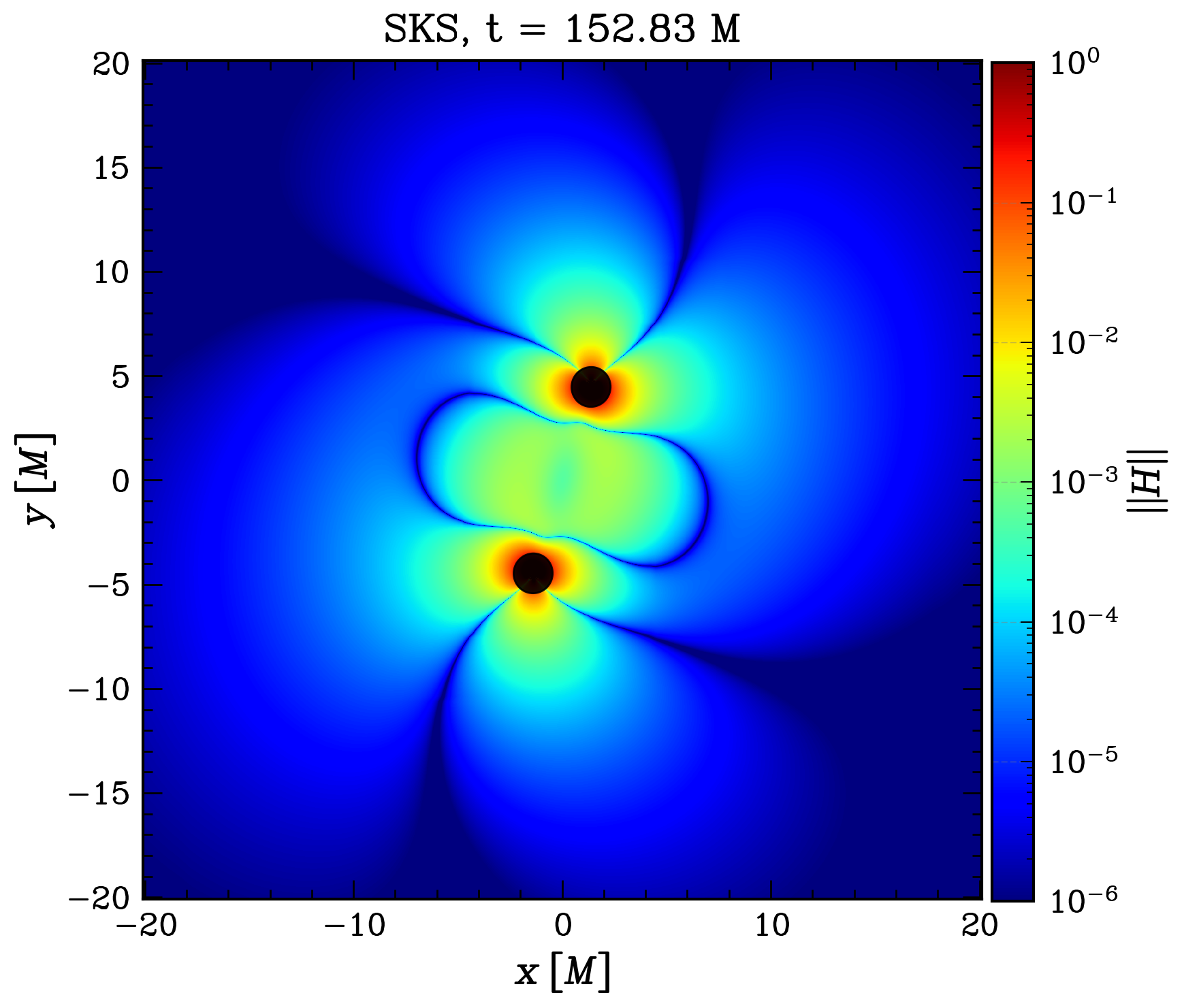
In solving Einstein’s equations, different sources of numerical error introduce violations to these constraints which can spoil the solution if they are not under control [101]. For an exact solution, the values of the constraint calculated numerically depend on the resolution. In contrast, because of the approximated nature of our SKS metric the constraints will not converge to zero with resolution. A local measure of (Equation 20) indicates the relative quality of the approximation for different points in space and time. Violations to the constraints, , can be interpreted as deviations from a vacuum solution of GR by the presence of a spurious rest-mass density. To quantify the global quality of the metric, we use the 1-norm and 2-norm of . The 1-norm of the constraints can be interpreted as the ‘fake’ mass introduced by the approximation. These quantities should be negligible compared to the total mass of the spacetime. One can also compare these numbers with the constraint violations for an exact solution at the same resolution (in our case, the norm of the constraint for the exact Kerr metric is given by )).
In Fig. 2 we show an equatorial snapshot of the Hamiltonian constraints at a particular time for Run-SKS and Run-BSSN. For Run-SKS, the highest values of the constraints violations are located near the black hole horizons, as well as the region between them (). In this region, the values of the constraint increase as the BHs approach each other. The bulk of the constraint violations are restricted to the orbital region and decrease rapidly outwards as . For Run-BSSN, the constraint violations are also concentrated in the orbital region but are more diffuse and the highest constraint violations are , lower in magnitude than those in Run-SKS.
In Fig. 3, we compare the 1-norm and 2-norm of the Hamiltonian constraints for Run-SKS and Run-BSSN. Both and remain almost constant for Run-SKS during inspiral up to the merger, where it drops orders of magnitude as the metric transition to the exact solution of the remnant black hole. This final value is determined by resolution. For the Run-BSSN, and increases a few orders of magnitude with respect to the initial data settling down after . We find that for the SKS metric is higher than the BSSN metric by one order of magnitude showing that locally, on average, constraints are lower for the BSSN metric. The total amount of constraints, quantified by , is higher for the BSSN metric because numerical violations propagate through all the domain.
IV.2.2 Apparent horizon formation and quasi-local properties

The SKS metric approximation is a strong field representation of the BH, e.g. different from a PN metric approximation [33]. To characterize the BHs and their properties (quasi-)locally, we resort to the concept of apparent horizon. An apparent horizon is defined as the outermost marginally trapped surface in a spatial slice; a marginally trapped surface is a closed 2-surface with future-pointing outgoing null geodesics having zero expansion:
| (22) |
We use the methods developed in Ref.[86] and implemented in the AHFinderDirect code to find and characterize the horizons in Run-SKS and Run-BSSN. In Fig. 4 we plot the (coordinate) separation of the binary measured from the centroid of the apparent horizons as a function of time for both Run-SKS and Run-BSSN. For Run-SKS, the apparent horizons follow naturally the PN trajectories we use for the boost. Besides the small eccentricity in the initial data, we see a very good agreement with Run-BSSN all the way up to the merger. They differ only in the last orbit, where Run-BSSN has one more orbital cycle; this is expected since the size of the horizon is larger for Run-SKS and the PN approximation is less accurate.
Because of the gauge differences that we pointed out before, the coordinate radius of the horizon inRun-SKS and Run-BSSN are different during evolution, as can be seen in the equatorial plane in Fig. 5, where Run-SKS horizons are bigger. The shape of the horizons found self-consistently through Eq. (22), barely changes during the inspiral. Remarkably, in Run-SKS we found a common apparent horizon once the separation of the black holes is sufficiently small () just before the interpolation to merger. The emergence of a third common apparent horizon is an expected feature of a binary merger [102, 103] and is also found in our Run-BSSN simulation. During the transition to the final remnant BH in Run-SKS, this common horizon evolves smoothly to the horizon of a Kerr-Schild black hole, as we interpolate the mass and spin.
As the separation of the binary gets smaller and smaller, the SKS approximation becomes less accurate. The expected properties of the binary merger are, nevertheless, reproduced by the approximation, i.e. two BH horizons evolve up to merger and form a common apparent horizon which relaxes to a final remnant Kerr BH. The quasi-local properties of the horizon are also well-behaved during evolution. To see this, we plot in Figure 6 the irreducible mass of one of the BHs for Run-SKS and Run-BSSN, defined simply as the where is the aerial radius of the apparent horizon. For Run-BSSN, the mass of one black hole is constant to during the entire simulation. In Run-SKS, the mass increases as the approximation worsens but only on level before merger. At merger, the mass settles to a final value of for Run-SKS (calculated from numerical relativity fitting formulae) and for Run-BSSN. The final spin measured at the horizon [104, 105] for Run-SKS and for Run-BSSN.
IV.3 Uniform plasma evolution onto binary black holes
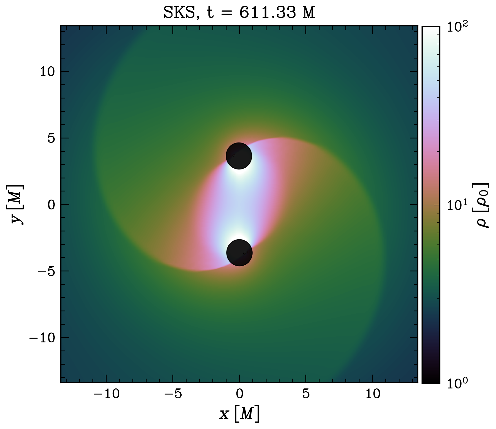

To show that the SKS metric is a good approximation for accretion physics even at very small separations, we evolve an initially static uniform gas onto the spacetime. This resembles a Bondi flow problem, which has been investigated for BH binaries [106, 47, 107]. For this system, the Bondi radius is given by .
After a short radially infalling phase, the flow reaches a quasi-steady state as can be seen in the accretion rate evolution onto the BHs in Fig. 8. Close to the black holes, the flow resembles a Bondi-Hoyle-Lyttleton fluid solution [108], with a shock front that propagates in the direction of motion of the black holes, creating spiral waves due to the orbital motion of the binary. In between the black holes, a tidal bridge is formed creating a stationary high-density region.
All these features are remarkably similar for Run-SKS and Run-BSSN even one orbit before the merger, as shown, e.g., in the equatorial density in Fig. 7. We find that Run-SKS has higher density regions near the horizon, by a factor of a few, while the flow velocity in Run-BSSN is slightly higher (see Fig.8). The accretion rate measured at the event horizon , where is the radial four-velocity in the BH frame, however, follows the same behavior in both simulations: it rises in the first , reaching a steady state that lasts until merger, when it settles into a new steady state very quickly. We observe only tens of percent differences between the accretion rates in each simulation. The specific energy of the flow averaged over the horizon differs by a factor of two, although this quantity is strongly gauge-dependent, especially near the horizon. The average velocity of the flow onto the horizon follows the same behavior in each run but differs throughout the beginning by a fixed constant offset that could be attributed to gauge differences in how we measure the velocity.

V Conclusions
We have presented a new general approximation for a binary black hole spacetime which accounts for arbitrary spins, eccentricities, and mass ratios. The new approximation is an excellent approximation for the inspiral regime and can be used even through merger, where we interpolate the metric to a BH remnant with properties obtained from NR fittings. We tested this approximation by analyzing its spacetime properties and performing a GRMHD simulation of uniform gas evolving on this dynamical metric background. We compare these results with a full numerical relativity simulation from small separations up to the merger. Our main results can be summarized as follows:
-
•
The SKS approximation is well-behaved through inspiral and merger. The norm of the Hamiltonian constraint violations remains constant during the entire evolution (Fig. 3), increasing locally between the black holes as the separation shortens (Fig.3). We show that the black hole trajectories, calculated using a 4PN approximation, follow the numerical relativity trajectory of the BHs quite well up to merger, see Fig. 4.
-
•
When the BHs reach separations of , we show that the SKS metric develops a common apparent horizon that relaxes smoothly to the remnant Kerr black hole horizon (Fig. 5). The mass of the BHs in Run-SKS, measured as the irreducible mass of the horizons, remains almost constant except in the last orbit before merger when it increases (Fig. 6).
-
•
We perform GRHD (GRMHD with very low magnetization) simulations using the SKS metric and a full numerical relativity evolution of Einstein’s equation with the BSSN formalism and puncture gauge. We show that the gas flow behaves qualitatively and quantitatively similarly in both cases, with differences of only tens of percent in the accretion onto the BHs that amount to a fixed constant.
-
•
We show that GRMHD simulations using the SKS metric as a background spacetime are much more efficient than a full numerical relativity evolution. Because the coordinate size of the horizon is larger and we do not have strict time convergence requirements in GRMHD compared to numerical relativity, we can evolve the GRMHD equations using less resolution and a second-order instead of a fourth-order Runge-Kutta time integrator. In addition, by evolving the spacetime only every 10 iterations (for a Courant factor of ), and not having to calculate and communicate all BSSN variables, we increase the efficiency by a factor of 5. Using the same grid and time integrator, the efficiency is still quite good, of the order of times faster.
Our analytical metric can be useful to explore regimes that are prohibitively expensive in numerical relativity such as small mass ratios and large separations. The numerical implementation of the SKS is public and can be found in a public repository [72] with the PN solver and Mathematica notebooks included. We are also planning to make public our implementation of the metric in the GR version of the Athena++ code as well as a module (thorn) for the EinsteinToolkit. We appreciate it if readers could point out bugs or mistakes in the implementation if found.
Acknowledgements.
LC would like to thank Manuela Campanelli, Carlos Lousto, and Luis Lehner for their support and ideas for this work. We thank Raphael Mignon-Risse for discussions, testing the metric, and pointing out some bugs. We also thank Geoff Ryan, Edu Gutierrez, Scott Noble, Will East, Erik Schnetter, and Joaquin Pelle for useful conversations. This research was enabled in part by support provided by SciNet (www.scinethpc.ca) and Compute Canada (www.computecanada.ca). We also acknowledge the support of the Natural Sciences and Engineering Research Council of Canada (NSERC), [funding reference number 568580] Cette recherche a été financée par le Conseil de recherches en sciences naturelles et en génie du Canada (CRSNG), [numéro de référence 568580]. Research at Perimeter Institute is supported in part by the Government of Canada through the Department of Innovation, Science and Economic Development Canada and by the Province of Ontario through the Ministry of Colleges and Universities.Appendix A Time-dependent boost transformation
To transform our BH superposed terms we need to invert the Fermi coordinate transformation which is defined from global (inertial) coordinates to BH (accelerated) coordinates . If the frame was moving on a uniform trajectory, this transformation and its inverse would be simply a Lorentz boost. For an arbitrary accelerated frame, we need in principle to solve a non-linear equation to obtain the inverse since the trajectory can depend non-linearly on time. We can however take the following approximation: expanding the trajectory around the global time we obtain . This approximation is good if is small in the transformation. Using the first Equation in (7) we have that ; for a fixed position in space, the error is then proportional to , which is small for a binary black hole orbit (). On the other hand, even though this term grows as we move away from the origin, the actual position of the black holes becomes irrelevant for the transformation at larger distances given that the orbit is bound; in other words, we have that as ,
Now, using this assumption and rewriting things as , with , we can write transformation in Eq. (7) in a form very similar to linear Lorentz boost plus a spatial displacement
| (23) | ||||
| (24) | ||||
| (25) | ||||
| (26) |
In this form, we can invert the system of equations by applying the inverse Lorentz matrix to obtain:
To find the Jacobian of this transformation, if we discard all acceleration terms , we have that , since and then it is easy to see that . Also notice that for a uniformly moving body, the transformation reduces directly to a linear boost since in that case. To obtain the explicit transformation given in Eq. (8), we can expand , and show that all linear dependence in time disappears from the transformation.
References
- Abbott et al. [2017] B. P. Abbott et al., ApJL 848, L13 (2017).
- Kelly et al. [2021] B. J. Kelly, Z. B. Etienne, J. Golomb, J. D. Schnittman, J. G. Baker, S. C. Noble, and G. Ryan, Phys. Rev. D 103, 063039 (2021), arXiv:2010.11259 [astro-ph.HE] .
- Bogdanović et al. [2022] T. Bogdanović, M. C. Miller, and L. Blecha, Living Reviews in Relativity 25, 3 (2022).
- Begelman et al. [1980] M. C. Begelman, R. D. Blandford, and M. J. Rees, Nature 287, 307 (1980).
- Artymowicz and Lubow [1996] P. Artymowicz and S. H. Lubow, ApJ 467, L77 (1996).
- Peters and Mathews [1963] P. C. Peters and J. Mathews, Phys. Rev. 131, 435 (1963).
- Peters [1964] P. C. Peters, Phys. Rev. 136, B1224 (1964).
- Afzal et al. [2023] A. Afzal, G. Agazie, A. Anumarlapudi, A. M. Archibald, Z. Arzoumanian, P. T. Baker, B. Bécsy, J. J. Blanco-Pillado, L. Blecha, K. K. Boddy, et al., The Astrophysical Journal Letters 951, L11 (2023).
- Agazie et al. [2023] G. Agazie, A. Anumarlapudi, A. M. Archibald, P. T. Baker, B. Bécsy, L. Blecha, A. Bonilla, A. Brazier, P. R. Brook, S. Burke-Spolaor, et al., arXiv preprint arXiv:2306.16220 (2023).
- Amaro-Seoane et al. [2017] P. Amaro-Seoane, H. Audley, S. Babak, J. Baker, E. Barausse, P. Bender, E. Berti, P. Binetruy, M. Born, D. Bortoluzzi, J. Camp, C. Caprini, V. Cardoso, M. Colpi, J. Conklin, N. Cornish, C. Cutler, K. Danzmann, R. Dolesi, L. Ferraioli, V. Ferroni, E. Fitzsimons, J. Gair, L. Gesa Bote, D. Giardini, F. Gibert, C. Grimani, H. Halloin, G. Heinzel, T. Hertog, M. Hewitson, K. Holley-Bockelmann, D. Hollington, M. Hueller, H. Inchauspe, P. Jetzer, N. Karnesis, C. Killow, A. Klein, B. Klipstein, N. Korsakova, S. L. Larson, J. Livas, I. Lloro, N. Man, D. Mance, J. Martino, I. Mateos, K. McKenzie, S. T. McWilliams, C. Miller, G. Mueller, G. Nardini, G. Nelemans, M. Nofrarias, A. Petiteau, P. Pivato, E. Plagnol, E. Porter, J. Reiche, D. Robertson, N. Robertson, E. Rossi, G. Russano, B. Schutz, A. Sesana, D. Shoemaker, J. Slutsky, C. F. Sopuerta, T. Sumner, N. Tamanini, I. Thorpe, M. Troebs, M. Vallisneri, A. Vecchio, D. Vetrugno, S. Vitale, M. Volonteri, G. Wanner, H. Ward, P. Wass, W. Weber, J. Ziemer, and P. Zweifel, arXiv e-prints , arXiv:1702.00786 (2017), arXiv:1702.00786 [astro-ph.IM] .
- Graham et al. [2015] M. J. Graham, S. Djorgovski, D. Stern, A. J. Drake, A. A. Mahabal, C. Donalek, E. Glikman, S. Larson, and E. Christensen, Monthly Notices of the Royal Astronomical Society 453, 1562 (2015).
- Charisi et al. [2016] M. Charisi, I. Bartos, Z. Haiman, A. M. Price-Whelan, M. J. Graham, E. C. Bellm, R. R. Laher, and S. Márka, MNRAS 463, 2145 (2016), arXiv:1604.01020 [astro-ph.GA] .
- Roedig et al. [2014] C. Roedig, J. H. Krolik, and M. C. Miller, The Astrophysical Journal 785, 115 (2014).
- MacFadyen and Milosavljević [2008] A. I. MacFadyen and M. Milosavljević, ApJ 672, 83 (2008), arXiv:astro-ph/0607467 [astro-ph] .
- Noble et al. [2012a] S. C. Noble, B. C. Mundim, H. Nakano, J. H. Krolik, M. Campanelli, Y. Zlochower, and N. Yunes, The Astrophysical Journal 755, 51 (2012a).
- Shi et al. [2012] J.-M. Shi, J. H. Krolik, S. H. Lubow, and J. F. Hawley, ApJ 749, 118 (2012), arXiv:1110.4866 [astro-ph.HE] .
- Bowen et al. [2017] D. B. Bowen, M. Campanelli, J. H. Krolik, V. Mewes, and S. C. Noble, ApJ 838, 42 (2017), arXiv:1612.02373 [astro-ph.HE] .
- Ryan and MacFadyen [2017] G. Ryan and A. MacFadyen, ApJ 835, 199 (2017), arXiv:1611.00341 [astro-ph.HE] .
- Westernacher-Schneider et al. [2021] J. R. Westernacher-Schneider, J. Zrake, A. MacFadyen, and Z. Haiman, arXiv e-prints , arXiv:2111.06882 (2021), arXiv:2111.06882 [astro-ph.HE] .
- D’Orazio et al. [2013] D. J. D’Orazio, Z. Haiman, and A. MacFadyen, Monthly Notices of the Royal Astronomical Society 436, 2997 (2013), arXiv:1210.0536 [astro-ph.GA] .
- Komossa [2006] S. Komossa, MmSAI 77, 733 (2006).
- Suková et al. [2021] P. Suková, M. Zajaček, V. Witzany, and V. Karas, ApJ 917, 43 (2021), arXiv:2102.08135 [astro-ph.HE] .
- Lehto and Valtonen [1996] H. J. Lehto and M. J. Valtonen, ApJ 460, 207 (1996).
- Britzen et al. [2023] S. Britzen, M. Zajaček, C. Fendt, E. Kun, F. Jaron, A. Sillanpää, A. Eckart, et al., ApJ 951, 106 (2023).
- Dittmann et al. [2023] A. J. Dittmann, A. M. Dempsey, and H. Li, arXiv preprint arXiv:2310.03832 (2023).
- Franchini et al. [2023] A. Franchini, M. Bonetti, A. Lupi, G. Miniutti, E. Bortolas, M. Giustini, M. Dotti, A. Sesana, R. Arcodia, and T. Ryu, Astronomy & Astrophysics 675, A100 (2023).
- Muñoz et al. [2020] D. J. Muñoz, D. Lai, K. Kratter, and R. Miranda, The Astrophysical Journal 889, 114 (2020).
- Miranda et al. [2017] R. Miranda, D. J. Muñoz, and D. Lai, MNRAS 466, 1170 (2017), arXiv:1610.07263 [astro-ph.SR] .
- Duffell et al. [2024] P. C. Duffell, A. J. Dittmann, D. J. D’Orazio, A. Franchini, K. M. Kratter, A. B. Penzlin, E. Ragusa, M. Siwek, C. Tiede, H. Wang, et al., arXiv preprint arXiv:2402.13039 (2024).
- Cattorini and Giacomazzo [2023] F. Cattorini and B. Giacomazzo, Astroparticle Physics , 102892 (2023).
- Gold [2019] Gold, Galaxies 7, 63 (2019).
- Noble et al. [2012b] S. C. Noble, B. C. Mundim, H. Nakano, J. H. Krolik, M. Campanelli, Y. Zlochower, and N. Yunes, Astrophys. J. 755, 51 (2012b), arXiv:1204.1073 [astro-ph.HE] .
- Zilhao et al. [2015] M. Zilhao, S. C. Noble, M. Campanelli, and Y. Zlochower, Phys. Rev. D91, 024034 (2015), arXiv:1409.4787 [gr-qc] .
- Noble et al. [2021] S. C. Noble, J. H. Krolik, M. Campanelli, Y. Zlochower, B. C. Mundim, H. Nakano, and M. Zilhão, arXiv preprint arXiv:2103.12100 (2021).
- Mundim et al. [2014] B. C. Mundim, H. Nakano, N. Yunes, M. Campanelli, S. C. Noble, and Y. Zlochower, Phys. Rev. D 89, 084008 (2014).
- Ireland et al. [2016] B. Ireland, B. C. Mundim, H. Nakano, and M. Campanelli, Physical Review D 93, 104057 (2016).
- Bowen et al. [2019] D. B. Bowen, V. Mewes, S. C. Noble, M. Avara, M. Campanelli, and J. H. Krolik, ApJ 879, 76 (2019), arXiv:1904.12048 [astro-ph.HE] .
- Avara et al. [2023] M. J. Avara, J. H. Krolik, M. Campanelli, S. C. Noble, D. Bowen, and T. Ryu, arXiv preprint arXiv:2305.18538 (2023).
- Mignon-Risse et al. [2023] R. Mignon-Risse, P. Varniere, and F. Casse, Monthly Notices of the Royal Astronomical Society 520, 1285 (2023).
- Farris et al. [2011] B. D. Farris, Y. T. Liu, and S. L. Shapiro, PhRvD 84, 024024 (2011), arXiv:1105.2821 .
- Farris et al. [2012] B. D. Farris, R. Gold, V. Paschalidis, Z. B. Etienne, and S. L. Shapiro, Phys. Rev. Lett. 109, 221102 (2012), arXiv:1207.3354 [astro-ph.HE] .
- Combi et al. [2021] L. Combi, F. G. L. Armengol, M. Campanelli, B. Ireland, S. C. Noble, H. Nakano, and D. Bowen, Physical Review D 104, 044041 (2021).
- Armengol et al. [2021] F. G. L. Armengol, L. Combi, M. Campanelli, S. C. Noble, J. H. Krolik, D. B. Bowen, M. J. Avara, V. Mewes, and H. Nakano, The Astrophysical Journal 913, 16 (2021).
- Gutiérrez et al. [2022] E. M. Gutiérrez, L. Combi, S. C. Noble, M. Campanelli, J. H. Krolik, F. L. Armengol, and F. García, The Astrophysical Journal 928, 137 (2022).
- Davelaar and Haiman [2022a] J. Davelaar and Z. Haiman, Physical Review D 105, 103010 (2022a).
- Davelaar and Haiman [2022b] J. Davelaar and Z. Haiman, Physical Review Letters 128, 191101 (2022b).
- Giacomazzo et al. [2012] B. Giacomazzo, J. G. Baker, M. C. Miller, C. S. Reynolds, and J. R. van Meter, The Astrophysical Journal 752, L15 (2012).
- Gold et al. [2014] R. Gold, V. Paschalidis, M. Ruiz, S. L. Shapiro, Z. B. Etienne, and H. P. Pfeiffer, Phys. Rev. D 90, 104030 (2014), arXiv:1410.1543 [astro-ph.GA] .
- Paschalidis et al. [2021] V. Paschalidis, J. Bright, M. Ruiz, and R. Gold, The Astrophysical Journal Letters 910, L26 (2021).
- Gold et al. [2014] R. Gold, V. Paschalidis, Z. B. Etienne, S. L. Shapiro, and H. P. Pfeiffer, Physical Review D 89, 10.1103/physrevd.89.064060 (2014).
- Kelly et al. [2017] B. J. Kelly, J. G. Baker, Z. B. Etienne, B. Giacomazzo, and J. Schnittman, Phys. Rev. D 96, 123003 (2017).
- Ressler et al. [2024] S. Ressler, L. Combi, X. Li, B. Ripperda, and H. Yang, Accepted in ApJ (2024).
- Poisson [2004] E. Poisson, A relativist’s toolkit: the mathematics of black-hole mechanics (Cambridge university press, 2004).
- Ma et al. [2021] S. Ma, M. Giesler, M. Scheel, and V. Varma, PhRvD 103, 084029 (2021), arXiv:2102.06618 .
- Fermi [1965] E. Fermi, in Enrico Fermi, Collected Papers (Note e Memorie) (Chicago University Press, Chicago, 1962–1965).
- Synge [1960] J. L. Synge, ed., Relativity: The General Theory (Interscience Publishers, New York,, 1960).
- Manasse and Misner [1963] F. Manasse and C. W. Misner, Journal of mathematical physics 4, 735 (1963).
- Poisson et al. [2011] E. Poisson, A. Pound, and I. Vega, Living Reviews in Relativity 14, 7 (2011).
- Mashhoon and Muench [2002] B. Mashhoon and U. Muench, Annalen der Physik 11, 532 (2002).
- Rindler [1956] W. Rindler, Monthly Notices of the Royal Astronomical Society 116, 662 (1956).
- Kidder [1995] L. E. Kidder, Physical Review D 52, 821 (1995).
- Csizmadia et al. [2012] P. Csizmadia, G. Debreczeni, I. Rácz, and M. Vasúth, Classical and Quantum Gravity 29, 245002 (2012).
- Note [1] cbwave.
- Blanchet [2014] L. Blanchet, Living reviews in relativity 17, 1 (2014).
- Kacskovics and Vasúth [2022] B. Kacskovics and M. Vasúth, Classical and Quantum Gravity 39, 095007 (2022).
- Buonanno et al. [2008] A. Buonanno, L. E. Kidder, and L. Lehner, Physical Review D 77, 026004 (2008).
- Lehner and Pretorius [2014] L. Lehner and F. Pretorius, Annual Review of Astronomy and Astrophysics 52, 661 (2014).
- Gerosa and Kesden [2016] D. Gerosa and M. Kesden, Physical Review D 93, 124066 (2016).
- Barausse et al. [2012] E. Barausse, V. Morozova, and L. Rezzolla, The Astrophysical Journal 758, 63 (2012).
- Hofmann et al. [2016] F. Hofmann, E. Barausse, and L. Rezzolla, The Astrophysical Journal Letters 825, L19 (2016).
- Kesden et al. [2010] M. Kesden, U. Sperhake, and E. Berti, Physical Review D 81, 084054 (2010).
- Combi and Ressler [2024] L. Combi and S. Ressler, Semi-analytical metric approximation of a binary black hole spacetime (2024).
- Combi et al. [2022] L. Combi, F. G. L. Armengol, M. Campanelli, S. C. Noble, M. Avara, J. H. Krolik, and D. Bowen, The Astrophysical Journal 928, 187 (2022).
- Nakamura et al. [1987] T. Nakamura, K. Oohara, and Y. Kojima, Prog. Theor. Phys. Suppl. 90, 1 (1987).
- Shibata and Nakamura [1995] M. Shibata and T. Nakamura, PhRvD 52, 5428 (1995).
- Baumgarte and Shapiro [1999] T. W. Baumgarte and S. L. Shapiro, PhRvD 59, 024007 (1999).
- Lichnerowicz [1944] A. Lichnerowicz, Bulletin de la Société Mathématique de France 72, 146 (1944).
- Arnowitt et al. [2008] R. L. Arnowitt, S. Deser, and C. W. Misner, Gen. Rel. Grav. 40, 1997 (2008).
- Baumgarte and Shapiro [2010] T. Baumgarte and S. Shapiro, Numerical Relativity (Cambridge University Press, Cambridge, 2010).
- Bona et al. [1995] C. Bona, J. Masso, E. Seidel, and J. Stela, PhRvL 75, 600 (1995).
- Alcubierre et al. [2003] M. Alcubierre, B. Bruegmann, P. Diener, M. Koppitz, D. Pollney, E. Seidel, and R. Takahashi, PhRvD 67, 084023 (2003).
- Goodale et al. [2003] T. Goodale, G. Allen, G. Lanfermann, J. Massó, T. Radke, E. Seidel, and J. Shalf, in High Performance Computing for Computational Science — VECPAR 2002, edited by J. M. L. M. Palma, A. A. Sousa, J. Dongarra, and V. Hernández (Springer Berlin Heidelberg, Berlin, Heidelberg, 2003) pp. 197–227.
- Loffler et al. [2012] F. Loffler et al., Cl. Quant Grav 29, 115001 (2012).
- Babiuc-Hamilton et al. [2019] M. Babiuc-Hamilton, S. R. Brandt, P. Diener, M. Elley, Z. Etienne, G. Ficarra, R. Haas, H. Witek, M. Alcubierre, D. Alic, et al., Zenodo (2019).
- Schnetter et al. [2004] E. Schnetter, S. H. Hawley, and I. Hawke, Cl. Quant Grav 21, 1465 (2004).
- Thornburg [2004] J. Thornburg, Cl. Quantum Grav 21, 743 (2004).
- Mösta et al. [2013] P. Mösta, B. C. Mundim, J. A. Faber, R. Haas, S. C. Noble, T. Bode, F. Löffler, C. D. Ott, C. Reisswig, and E. Schnetter, Class. Quantum Grav. 31, 015005 (2013).
- Combi and Siegel [2023] L. Combi and D. M. Siegel, The Astrophysical Journal 944, 28 (2023).
- Baiotti et al. [2005] L. Baiotti, I. Hawke, P. J. Montero, F. Loffler, L. Rezzolla, N. Stergioulas, J. A. Font, and E. Seidel, PhRvD 71, 024035 (2005).
- Brown et al. [2009] J. D. Brown, P. Diener, O. Sarbach, E. Schnetter, and M. Tiglio, Phys. Rev. D79, 044023 (2009), arXiv:0809.3533 [gr-qc] .
- Ansorg et al. [2004] M. Ansorg, B. Bruegmann, and W. Tichy, Phys. Rev. D70, 064011 (2004), arXiv:gr-qc/0404056 [gr-qc] .
- Brandt and Brügmann [1997] S. Brandt and B. Brügmann, Physical Review Letters 78, 3606 (1997).
- Gourgoulhon [2007] E. Gourgoulhon, in Journal of Physics: Conference Series, Vol. 91 (IOP Publishing, 2007) p. 012001.
- Font et al. [2002] J. A. Font, T. Goodale, S. Iyer, M. A. Miller, L. Rezzolla, E. Seidel, N. Stergioulas, W.-M. Suen, and M. Tobias, PhRvD 65, 084024 (2002).
- Harten et al. [1987] A. Harten, B. Engquist, S. Osher, and S. R. Chakravarthy, J. Comput. Phys. 71, 231 (1987).
- Tchekhovskoy et al. [2007] A. Tchekhovskoy, J. C. McKinney, and R. Narayan, MNRAS 379, 469 (2007).
- Siegel et al. [2018] D. M. Siegel, P. Mösta, D. Desai, and S. Wu, ApJ 859, 71 (2018).
- White et al. [2016] C. J. White, J. M. Stone, and C. F. Gammie, The Astrophysical Journal Supplement Series 225, 22 (2016).
- Sadiq et al. [2018] J. Sadiq, Y. Zlochower, and H. Nakano, Physical Review D 97, 084007 (2018).
- Baumgarte and Naculich [2007] T. W. Baumgarte and S. G. Naculich, Physical Review D 75, 067502 (2007).
- Alic et al. [2013] D. Alic, W. Kastaun, and L. Rezzolla, PhRvD 88, 064049 (2013).
- Hawking and Ellis [2023] S. W. Hawking and G. F. Ellis, The large scale structure of space-time (Cambridge university press, 2023).
- Pook-Kolb et al. [2021] D. Pook-Kolb, R. A. Hennigar, and I. Booth, Physical Review Letters 127, 181101 (2021).
- Dreyer et al. [2003] O. Dreyer, B. Krishnan, D. Shoemaker, and E. Schnetter, Phys. Rev. D67, 024018 (2003), arXiv:gr-qc/0206008 [gr-qc] .
- Schnetter et al. [2006] E. Schnetter, B. Krishnan, and F. Beyer, Physical Review D 74, 024028 (2006).
- Farris et al. [2010] B. D. Farris, Y. T. Liu, and S. L. Shapiro, Physical Review D 81, 084008 (2010).
- Cattorini et al. [2021] F. Cattorini, B. Giacomazzo, F. Haardt, and M. Colpi, Physical Review D 103, 103022 (2021).
- Edgar [2004] R. Edgar, New Astronomy Reviews 48, 843 (2004).