A biased dollar exchange model involving bank and debt with discontinuous equilibrium
Abstract
In this work, we investigate a biased dollar exchange model with collective debt limit, in which agents picked at random (with a rate depending on the amount of dollars they have) give at random time a dollar to another agent being picked uniformly at random, as long as they have at least one dollar in their pockets or they can borrow a dollar from a central bank if the bank is not empty. This dynamics enjoys a mean-field type interaction and partially extends the recent work [9] on a related model. We perform a formal mean-field analysis as the number of agents grows to infinity and as a by-product we discover a two-phase (ODE) dynamics behind the underlying stochastic -agents dynamics. Numerical experiments on the two-phase (ODE) dynamics are also conducted where we observe the convergence towards its unique equilibrium in the large time limit.
Key words: Econophysics, Agent-based model, Interacting agents, Mean-field, Two-phase, Bank
1 Introduction
Econophysics is a subfield of statistical physics that draw concepts and techniques from traditional physics and apply them to economics, finance, and related fields, and we refer the readers to the pioneer work [15] for many models motivated from econophysics. Among many important tasks in this area of research, a fundamental mission is to demystify how various (macroscopic) economical phenomena could be explained by (microscopic) laws in classical statistical physics under certain modeling assumptions, and we refer to [18, 25, 26, 27] for a general review on using kinetic theory for the modelling of wealth (re-)distributions.
Motivations for studying econophysics models are at least two-fold: from the perspective of a policy maker, how to exert influence on the growing wealth inequality in order to mitigate the alarming gap between rich and poor is a central issue to be dealt with. From a mathematical viewpoint, the underlying mechanisms behind the formation of macroscopic phenomena, for instance various possible wealth distributions arising from distinct agent-based dollar exchange models, remain to be thoroughly understood. For a given agent-based model, we aim at identifying a limit dynamics, which is fully deterministic, when we send the number of individuals/players to infinity, and then the deterministic system will be further analyzed with the hope of proving its convergence to equilibrium (if there is one) in the large time limit. This philosophy has been successfully implemented among the overabundant literatures across different fields of applied mathematics, see for instance [7, 2, 10, 24].
In this work, we consider a simple mechanism for money exchange involving a bank, meaning that there are a fixed number of agents (denoted by ) and one bank. We denote by the amount of dollars the agent has at time and we suppose that for some fixed . Thus, each agent in this closed economic system has dollars on average. Moreover, we denote by the initial amount of dollars in the bank, where and represent the amount of dollars owned by the bank in the form of “cash” and in the form of “debt” (borrowed by agents), respectively. Also, we introduce another parameter , which measures the ratio of the bank’s initial wealth to the initial combined wealth of all the agents, and set to be the total amount of dollars put in the bank initially. We emphasize here that the parameters and are both dimensionless constants.
The model investigated in this work was a natural variant of the model proposed in [30] and revisited in several recent works [9, 21], which we now briefly recall first: at random times (generated by an exponential law), an agent (the “giver”) and an agent (the “receiver”) are picked uniformly at random. If either the “giver” has at least one dollar (i.e. ) or if the central bank has “cash” (i.e. ), then the receiver receives a dollar. Otherwise, when the giver has no dollar and the bank has no cash, then nothing happens. To further clarify the aforementioned model, we emphasize that dollars in the central bank are untouched when the giver has at least one dollar, and the giver will borrow a dollar from the bank (as long as the bank has money) if he/she has no dollar to give. The aforementioned model is termed as the unbiased exchange model with collective debt limit in [9] and the one-coin model with collective debt limit in [21]. Notice that when the bank gives a dollar to agent , there is still one dollar withdrew from the giver , i.e., the debt of agent increases. The debt of agent could be reduced once it will become a “receiver”. It is also important to notice that in this model the bank never loses money, it just transforms its “cash” into “debt” (and vice versa). Without the bank, agents can only give a dollar when they have at least one dollar (hence no debt is allowed).
We now introduce the model considered in the present manuscript as a biased version of the aforementioned model, i.e., we drop the rule of selecting the “giver” uniformly at random in favor of the requirement that the “giver” agent will be picked (at each jump time) at a rate proportional to , where is a strictly positive function. From now on, we terms the model as the -biased exchange model with collective debt limit, which can be represented by (1.1) below.
| (1.1) |
We emphasize that the unbiased exchange model with collective debt limit investigated in [9] is a special case of the model we introduced here where is a fixed positive constant (which can be normalized to without loss of generality). For now the function is an arbitrary positive function from to , but later we will impose appropriate constraints on for reasons to be further clarified in the subsequent development of our analysis.
Remark. In order to have the correct asymptotic as the number of agents goes to infinity , we need to adjust the rate by normalizing by , which amounts to replacing in (1.1) by so that the rate of a typical agent giving a dollar per unit time is of order . Here by saying “a typical agent” we mean an agent picked (uniformly) at random from the crowd of agents.
The fundamental problem of interest is the derivation/idenfication of the limiting money distribution among the agents as the total number of agents and time become large. We propose two analytical approaches for addressing this problem with illustration provided by figure 1 below. The first approach, detailed in section 2, relies on the study of the limiting money distribution for all (fixed) values of the number of agents as time goes to infinity and then simplification of the probability that a typical agent has dollars at (“thermodynamic”) equilibrium in the large population limit.

The second approach is a mean-field approach carried out in the spirit of the recent work [9], which will be presented in section 3. The first step in the mean-field approach lies in the derivation of its limit dynamics as the number of agents goes to infinity (i.e., ). With this goal, we introduce the probability distribution of dollars:
| (1.2) |
with . The evolution of will be given by a system of (deterministic) nonlinear ordinary differential equations. However, to rigorously justify the transition from a stochastic interacting agents systems into a deterministic set of ODEs, one needs the so-called propagation of chaos [28]. Heuristically speaking, the propagation of chaos property in the specific context of our model says that the (random) agent and agent picked to engage in the binary trading activity (1.1) are statistically independent as . The rigorous derivation of the mean-field ODE system (1.3) from its underlying stochastic -agents dynamics is out of the scope of the present paper, but the derivation has been fully justified in various models arising from econophysics, see for instance [4, 5, 6, 8, 14]. The major difficulty in the mean-field argument lies in the fact that the evolution of is split into two phases. Indeed, the evolution of changes at the first time when there is no more cash in the bank. We will denote by the time at which such event occur, i.e., at the bank is empty for the first time. We will show that the evolution equation for takes the following form
| (1.3) |
where the exact expressions for the operator and are given by (3.5) and (3.17), respectively. Once the large population limit has been carried out and a limit (deterministic) dynamics has been uncovered, one naturally attempts to investigate the asymptotic behavior of the probability mass function as , with the intent of proving convergence to the unique equilibrium distribution (if such unique equilibrium exists). Unfortunately, we do not aim to address the problem of the convergence to equilibrium for the two-phase ODE system (1.3) analytically, and we will be content with numerical evidence on such convergence behavior.
Although we will only investigate a specific binary dollar exchange model in the current work, other exchange rules can also be imposed and studied, leading to other econophysics models. To name a few, the so-called immediate exchange model introduced in [17] assumes that pairs of agents are randomly and uniformly picked at each random time, and each agent transfers a random fraction of their money to the other agent, where these fractions are independent and uniformly distributed on . The so-called uniform reshuffling model investigated in [5, 15, 20, 23] proposes that the total amount of money of two randomly and uniformly picked agents possessed before interaction is uniformly redistributed among the two agents after interaction. The so-called repeated averaging model studied for instance in [6] studies the mechanism where two randomly selected agents share half of their wealth with each other at each binary exchange. The binomial reshuffling model proposed in a recent work [3] is a variant of the uniform reshuffling mechanism in which the agents’ combined wealth is redistributed according to a binomial distribution. For models with saving propensity, models involving debts, or other econophysics models, we refer the readers to [1, 11, 12, 21, 9, 13, 16, 29] and the references therein.
2 Markov chain approach
In this section, we will tackle the problem of finding the limiting money distribution (as ) using the techniques employed in [19, 20, 21, 22]. Define to be the set of possible configurations with agents having a total initial wealth of dollars, where the initial amount of dollars in the bank equals , i.e.,
Let us fix any and introduce defined via
Then is a continuous-time Markov chain having state space . Note also that all transitions of the process are of the form for some .
As indicated in the introduction, the rates of transition from to with for the process are given by
We first show that is a finite, irreducible and aperiodic Markov chain, whence it admits a unique stationary distribution.
Lemma 2.1
The process has a unique stationary distribution such that
Proof.
Lemma 2.2
The process is reversible and has the stationary distribution given by
| (2.1) |
where
| (2.2) |
Proof.
We are now ready to state the following general convergence result, which follows readily from Lemmas 2.1 and 2.2.
Theorem 1
The fraction of agents with dollars in the long run, or equivalently the probability that a typical agent has dollars in the large time limit, is given by
| (2.6) |
From now on, we will take a “carefully crafted” nonlinear function , which is provided in the following definition.
Definition 1
We define to be for all and for .
The motivation to consider and treat this particular (“strange looking”) nonlinear is at least two-fold and will be elaborated in section 3 when we employ a mean-field approach. For the moment, we proceed with this specific choice of to deduce the following corollary.
Corollary 2.3
If is taken to be as in Definition 1, then .
Proof.
We now state some elementary identities from combinatorics, whose proofs are standard.
Lemma 2.4
For each and , we have
| (2.8) |
Proof.
is the number of integer solutions to with , which is known to be .
Lemma 2.5
We have for each and that
| (2.9) |
Proof.
For ease of writing, let us define
| (2.10) |
and
| (2.11) |
We shall prove the desired result with induction on .
Base Case: When or , then we have the following results for , , and .
and
Inductive Step: Assume that our hypothesis holds for all such that , and for some . Then setting and employing Pascal’s identity we have
and
Lemma 2.6
For each and ,
| (2.12) |
Proof.
We will show the desired result using induction on .
Base Case: . We have
Inductive Step: Assume that our hypothesis holds for where . Then setting and employing Lemma 2.5, we have that
Now we can specialize the content of Theorem 1 to deduce the following convergence result.
Corollary 2.7
If is taken to be as in Definition 1, set
| (2.13) |
then
Consequently, the distribution of dollars among the -agents system in the large time limit is given by
| (2.14) |
Proof.
If we define to be the weighted sum of over all configurations with agents, dollars of agents combined initial wealth, dollars in the bank initially, and with dollars of total debt and agents with less than or equal to zero dollars, then we have that
| (2.15) |
Remark. Even though the equilibrium distribution (for any fixed ) (2.14) is explicit in , it is a very hard task to take the large population limit (by using some basic algebraic manipulations) in order to simplify the expression for
| (2.17) |
We henceforth leave the computations/simplications of (2.17) as a open problem. On the other hand, we will employ the mean-field approach in the next section and deduce the explicit equilibrium distribution (for the choice ).
3 Formal mean-field limit
In this section, we carry out a formal mean-field argument of the stochastic agent-based dynamics (1.1) as the number of agents goes to infinity, following the procedure detailed in [9].
The biased exchange model with collective debt limit can be written in terms of a system of stochastic differential equations, thanks to the framework set up in [4, 9] for the study of the basic unbiased exchange model as well as some of its variants. Introducing , which represents a collection of independent Poisson processes with intensity , the evolution of each is given by:
| (3.1) |
where we use the notation . By the obvious symmetry, we can focus on the case when and notice that whenever , the SDE for simplifies to
| (3.2) |
If we introduce
then the two Poisson processes and are of intensities and , respectively. Motivated by (3.2), we give the following definition of the limiting dynamics of as from the process point of view, providing that .
Definition 2 (Mean-field equation — Phase I)
We define to be the compound Poisson process satisfying the following SDE:
| (3.3) |
in which and are independent Poisson processes with intensities and , where denotes the law of the process , i.e. .
Its time evolution is given by the following dynamics:
| (3.4) |
with
| (3.5) |
The distribution naturally preserves its mass (since it is a probability mass function) and the mean value (as the total amount of money in the whole system is preserved), thus if we introduce the affine subspaces:
| (3.6) |
and
then it is clear that the unique solution of (3.4)-(3.5) with satisfies for all . Moreover, we will introduce a class of functions by setting
| (3.7) |
If we define the average amount of “debt” per agent as
| (3.8) |
then this quantity will be non-decreasing for all since
| (3.9) | ||||
in which the last inequality follows directly from the assumption that .
Remark. The class of functions (at least) includes the following class of decreasing functions defined by
| (3.10) |
Indeed, if is decreasing and , we have
From now on, we will always impose the condition on the function unless otherwise stated. Since the average amount of debt each agent can sustain in the underlying stochastic -agents system is at most , we therefore terminate the evolution of Phase I (3.4)-(3.5) until , where
| (3.11) |
Remark. The primary reason for assuming that belongs to the class lies the desire to ensure that , which is a sufficient (but not necessarily) condition to guarantee that the Phase I will terminate at a finite time . It would be harder to show that the average amount of “debt” per agent will reach the threshold in finite time when is not assumed to be a member of .
At the level of the agent-based system, after the first time when there is no cash in the bank, i.e., when , the analysis is much more involved so heuristic reasoning plays a major role in this manuscript. We notice that we have the following basic relations for all time :
| (3.12) |
and . Therefore, the evolution of is much faster than the evolution of each of the ’s, indicating that (3.12) is really a “fast” dynamics compared to (3.1). These observations motivate the next definition:
Definition 3 (Mean-field equation — Phase II)
We define (for ) to be the compound Poisson process satisfying the following SDE:
| (3.13) |
in which and are independent Poisson processes with intensities and . Moreover, and are independent Bernoulli random variables with parameters
| (3.14) |
and
| (3.15) |
respectively.
We again denote by the law of the process for , i.e. for . Its time evolution is given by the following dynamics:
| (3.16) |
with
| (3.17) |
where
| (3.18) |
We remark here that and represent the proportion of “rich” and “indebted” agents, respectively.
Remark. We will illustrate the motivation behind Definition 3. Taking the large population limit , if we denote by the law of , then the transition rates of can be described by figure 2 below.

To be precise, the transition occurs at rate when a “rich” agent is being picked () and gives a dollar to an “indebted” agent (). Similarly, the transition occurs at rate when an agent without dollar is being picked () and gives a dollar to an agent without debt () and moreover . As the evolution of is a “fast” dynamics (compared to the evolution of each agents’ wealth), we assume that its distribution will converge to its ergodic invariant distribution within a time-scale that is negligible compared to the evolution of each of the ’s. Thus, from the following detailed balance equation at equilibrium
one arrives at for all . Due to identity , we deduce that
which coincides with the expression (3.15). Meanwhile, the transition rates of can be described by figure 3.

This suggests that the evolution of should obey
| (3.19) |
with
| (3.20) |
with . Thus, it is clear that the system (3.19)-(3.20) coincides with (3.16)-(3.17).
In Phase II, the average debt is preserved, therefore we can further restrict the affine space where the solution of (3.16)-(3.17) lives:
| (3.21) |
it is straightforward to check that if then for all .
We now turn to the search for the equilibrium distribution to (3.16)-(3.17). Indeed, if we denote by the equilibrium solution to (3.16)-(3.17), then for we have
leading to the conclusion that equals to the same constant for all . Similarly, we obtain that equals to the same constant for all . Therefore, for a general positive with , the “ansatz” for the equilibrium distribution takes the following form
| (3.22) |
in which and will be determined thought the following three constraints:
| (3.23) |
In particular, if we take where is given in Definition 1, so that for and for , then (3.22) simplifies to
| (3.24) |
Moreover, it is straightforward to check that . Taking into account of the constraints (3.23), we obtain
| (3.25a) | ||||
| (3.25b) | ||||
| (3.25c) | ||||
To solve the system of nonlinear equations (3.25), we proceed as follows. Substituting (3.25c) into (3.25b) yields that
| (3.26) |
Also, we can deduce from (3.25a) and (3.25c) that
| (3.27) |
and
| (3.28) |
Since , we have
| (3.29) |
Inserting (3.26) into (3.29) gives
which is equivalent to the following quartic equation (with only one unknown):
| (3.30) |
where
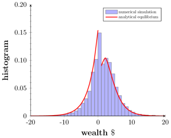
It is natural to speculate that the system of nonlinear equations (3.25) admits a unique solution for , for any prescribed . Unfortunately we can not provide a rigorous proof of this natural conjecture. As a comprise, we are dedicated to solving the nonlinear system (3.25) for specific choices of the pair . For instance, when , one can find that , , and . The agent-based numerical simulation suggests that, as the number of agents and time go to infinity, the limiting distribution of money approaches the equilibrium distribution (3.24) as shown in figure 4, in which we take .
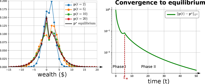
To illustrate the convergence of toward the equilibrium , we run a simulation and plot the evolution of at various times (see figure 5-left) as well as the evolution of the distance between and over time (see figure 5-right). We emphasize that the decay of the distance changes abruptly around which corresponds to the transition of the dynamics from phase I to phase II.
Remark. We now illustrate the main reasons for considering the “strange-looking” function . Indeed, for the mean-field approach developed in [9] to be applicable in our generalized setting (where is no longer a fixed positive constant), we need to ensure that the quantity (3.8) to be non-decreasing during Phase I so that we indeed have a two-phase dynamics. This consideration leads us to the restriction . For example, if one wants to take the function to be for and for , then an ansatz for the equilibrium distribution (3.22) boils down to
| (3.31) |
However, with this choice of it is no longer clear whether or not.
Second of all, we also need to ensure that our choice of leads to the existence of a equilibrium distribution associated with (3.16)-(3.17) in the space (3.21). For instance, let us take for some , which belongs to the class (3.10) but also approaches to infinity as . In this scenario, the equilibrium (3.22) takes the form
| (3.32) |
However, as , in the form of (3.32) has no chance to be a probability mass function and our analytical framework breaks down. Lastly, we want to make sure that our choice allows an explicit computation of the equilibrium at least for each fixed pair of the model parameters , this consideration takes into account of the possibility of simulating the stochastic -agents dynamics so that we can compare our analytical prediction with numerical observations. Putting together these concerns, we decide to pick to be as in Definition 1 in the majority part of the present paper.
4 Conclusion
In this manuscript, the so-called -biased exchange model with collective debt limit is investigated, which serves as an extension of the unbiased exchange model with collective debt limit proposed in [30] and revisited recently in [9, 21]. Although our generalized setting necessarily induces additional difficulty in the analysis using the framework developed in [9], we are delighted to find that our analytical prediction of the asymptotic wealth distribution among agents as and based on our two-phase dynamics (1.3) fits well with the numerical experiments, at least for a specific choice of the nonlinearity .
To the best our of knowledge, rigorous treatment of econophysics models involving bank and debt is relatively rare in the literature and we refer to [29] for some rigorous analysis on certain econophysics models at the PDE level (whence completely bypassing the need to investigate the large population limit at the agent-based level). Our work also leaves many important open questions to be addressed in subsequent studies. For instance, is it possible to derive the two-phase dynamics (1.3) rigorously ? Will it be possible to extend the framework developed in [9] so that analysis can be carried for broader class of functions (especially for whose functions ) ? For those belonging to the class such that indeed defines a probability distribution, can we show rigorously that the solution of the Phase II ODE system (3.16)-(3.17) converges to its equilibrium distribution ? We also emphasize that a rigorous study, based on the relative entropy, is possible when is assumed to a fixed positive constant [9]. Finally, for the Markov chain approach taken in section 2, will it be possible to simplify the expression (2.14) in Corollary 2.7 so that a closed and explicit form of the probability (2.17) can be discovered, perhaps by resorting to advanced combinatorics tools or approximation theories ? We believe that answers to many of these problems deserve separate and thorough investigations on their own.
Acknowledgement We highly appreciate the help from Sébastien Motsch on the generation of figure 5.
References
- [1] Bruce M.Boghosian, Merek Johnson, and Jeremy A. Marcq. An Theorem for Boltzmann’s Equation for the Yard-Sale Model of Asset Exchange: The Gini Coefficient as an Functional. Journal of Statistical Physics, 161:1339–1350, 2015.
- [2] Fei Cao. -averaging agent-based model: propagation of chaos and convergence to equilibrium. Journal of Statistical Physics, 184(2):1–19, 2021.
- [3] Fei Cao, and Nicholas F. Marshall. From the binomial reshuffling model to Poisson distribution of money. arXiv preprint arXiv:arXiv:2212.14388, 2022.
- [4] Fei Cao, and Sebastien Motsch. Derivation of wealth distributions from biased exchange of money. Kinetic & Related Models, 16(5):764–794, 2023.
- [5] Fei Cao, Pierre-Emannuel Jabin, and Sebastien Motsch. Entropy dissipation and propagation of chaos for the uniform reshuffling model. Mathematical Models and Methods in Applied Sciences, 33(4):829–875, 2023.
- [6] Fei Cao. Explicit decay rate for the Gini index in the repeated averaging model. Mathematical Methods in the Applied Sciences, 46(4):3583–3596, 2023.
- [7] Fei Cao, Sebastien Motsch, Alexander Reamy, and Ryan Theisen. Asymptotic flocking for the three-zone model. Mathematical Biosciences and Engineering, 17(6):7692–7707, 2020.
- [8] Fei Cao, and Pierre-Emannuel Jabin. From interacting agents to Boltzmann-Gibbs distribution of money. arXiv preprint arXiv:2208.05629, 2022.
- [9] Fei Cao, and Sebastien Motsch. Uncovering a two-phase dynamics from a dollar exchange model with bank and debt. SIAM Journal on Applied Mathematics, 83(5):1872–1891, 2023.
- [10] Eric Carlen, Pierre Degond, and Bernt Wennberg. Kinetic limits for pair-interaction driven master equations and biological swarm models. Mathematical Models and Methods in Applied Sciences, 23(07):1339–1376, 2013.
- [11] Anirban Chakraborti, and Bikas K. Chakrabarti. Statistical mechanics of money: how saving propensity affects its distribution. The European Physical Journal B-Condensed Matter and Complex Systems, 17(1):167–170, 2000.
- [12] Arnab Chatterjee, Bikas K. Chakrabarti, and Subhrangshu Sekhar Manna. Pareto law in a kinetic model of market with random saving propensity. Physica A: Statistical Mechanics and its Applications, 335(1-2):155–163, 2004.
- [13] David W. Cohen, and Bruce M. Boghosian. Bounding the approach to oligarchy in a variant of the yard-sale model. arXiv preprint arXiv:2310.16098, 2023.
- [14] Roberto Cortez, and Fei Cao. Uniform propagation of chaos for a dollar exchange econophysics model. arXiv preprint arXiv:2212.08289, 2022.
- [15] Adrian Dragulescu, and Victor M. Yakovenko. Statistical mechanics of money. The European Physical Journal B-Condensed Matter and Complex Systems, 17(4):723–729, 2000.
- [16] Bertram Düring, Daniel Matthes, and Giuseppe Toscani. Kinetic equations modelling wealth redistribution: a comparison of approaches. Physical Review E, 78(5):056103, 2008.
- [17] Els Heinsalu, and Patriarca Marco. Kinetic models of immediate exchange. The European Physical Journal B, 87(8):1–10, 2014.
- [18] Ryszard Kutner, Marcel Ausloos, Dariusz Grech, Tiziana Di Matteo, Christophe Schinckus, and H. Eugene Stanley. Econophysics and sociophysics: Their milestones & challenges. Physica A: Statistical Mechanics and its Applications, 516:240–253, 2019.
- [19] Nicolas Lanchier. Rigorous proof of the Boltzmann–Gibbs distribution of money on connected graphs. Journal of Statistical Physics, 167(1):160–172, 2017.
- [20] Nicolas Lanchier, and Stephanie Reed. Rigorous results for the distribution of money on connected graphs. Journal of Statistical Physics, 171(4):727–743, 2018.
- [21] Nicolas Lanchier, and Stephanie Reed. Rigorous results for the distribution of money on connected graphs (models with debts). Journal of Statistical Physics, 176(5):1115–1137, 2019.
- [22] Nicolas Lanchier, and Stephanie Reed. The role of cooperation in spatially explicit economical systems. Advances in Applied Probability, 50(3):743–758, 2018.
- [23] Daniel Matthes, and Giuseppe Toscani. On steady distributions of kinetic models of conservative economies. Journal of Statistical Physics, 130:1087-1117, 2008.
- [24] Sebastien Motsch, and Diane Peurichard. From short-range repulsion to Hele-Shaw problem in a model of tumor growth. Journal of Mathematical Biology, 76:205–234, 2018.
- [25] Lorenzo Pareschi, and Giuseppe Toscani. Interacting multiagent systems: kinetic equations and Monte Carlo methods. OUP Oxford, 2013.
- [26] Eder Johnson de Area Leão Pereira, Marcus Fernandes da Silva, and HB de B. Pereira. Econophysics: Past and present. Physica A: Statistical Mechanics and its Applications, 473:251–261, 2017.
- [27] Gheorghe Savoiu. Econophysics: Background and Applications in Economics, Finance, and Sociophysics. Academic Press, 2013.
- [28] Alain-Sol Sznitman. Topics in propagation of chaos. In Ecole d’été de probabilités de Saint-Flour XIX—1989, pages 165–251. Springer, 1991.
- [29] Marco Torregrossa, and Giuseppe Toscani. Wealth distribution in presence of debts. A Fokker-Planck description. arXiv preprint arXiv:1709.09858, 2017.
- [30] Ning Xi, Ning Ding, and Yougui Wang. How required reserve ratio affects distribution and velocity of money. Physica A: Statistical Mechanics and its Applications, 357(3-4):543–555, 2005. Publisher: Elsevier.