A Benchmark for Low-Switching-Cost Reinforcement Learning
Abstract
A ubiquitous requirement in many practical reinforcement learning (RL) applications, including medical treatment, recommendation system, education and robotics, is that the deployed policy that actually interacts with the environment cannot change frequently. Such an RL setting is called low-switching-cost RL, i.e., achieving the highest reward while reducing the number of policy switches during training. Despite the recent trend of theoretical studies aiming to design provably efficient RL algorithms with low switching costs, none of the existing approaches have been thoroughly evaluated in popular RL testbeds. In this paper, we systematically studied a wide collection of policy-switching approaches, including theoretically guided criteria, policy-difference-based methods, and non-adaptive baselines. Through extensive experiments on a medical treatment environment, the Atari games, and robotic control tasks, we present the first empirical benchmark for low-switching-cost RL and report novel findings on how to decrease the switching cost while maintain a similar sample efficiency to the case without the low-switching-cost constraint. We hope this benchmark could serve as a starting point for developing more practically effective low-switching-cost RL algorithms. We release our code and complete results in https://sites.google.com/view/low-switching-cost-rl.
1 Introduction
Reinforcement Learning (RL) has been successfully applied to solve sequential-decision problems in many real-world scenarios, such as medical domains [16], robotics [7, 12], hardware placements [20, 19], and personalized recommendation [28]. When performing RL training in these scenarios, it is often desirable to restrict the agent from adjusting its policy too often due to the high costs and risks of deployment. For example, updating a treatment strategy in medical domains requires a thorough approval process by human experts [2]; in personalized recommendations, it is impractical to adjust the policy online based on instantaneous data and a more common practice is to aggregate data in a period before deploying a new policy [28]; in problems where we use RL to learn hardware placements [20], it is desirable to limit the frequency of changes to the policy since it is costly to launch a large-scale evaluation procedure on hardware devices like FPGA; for learning to control a real robot, it may be risky or inconvenient to switch the deployed policy when an operation is being performed. In these settings, it is a requirement that the deployed policy, i.e., the policy used to interact with the environment, could keep unchanged as much as possible. Formally, we would like our RL algorithm to both produce a policy with the highest reward and at the same time reduce the number of deployed policy switches (i.e., a low switching cost) throughout the training process.
Offline reinforcement learning [15] is perhaps the most related framework in the existing literature that also has a capability of avoiding frequent policy deployment. Offline RL assumes a given transition dataset and performs RL training completely in an offline fashion without interacting with the environment at all. [18] adopt a slightly weaker offline assumption by repeating the offline training procedure, i.e., re-collecting transition data using the current policy and re-applying offline RL training on the collected data, for about 10 times. However, similar to the standard offline RL methods, due to such an extreme low-deployment-constraint, the proposed solution suffers from a particularly low sample efficiency and even produces significantly lower rewards than online SAC method in many cases [18]. In contrast with offline RL, which optimizes the reward subject to a minimal switching cost, low-switching-cost RL aims to reduce the switching cost while maintain a similar sample efficiency and final reward compared to its unconstrained RL counterpart.
In low-switching-cost RL, the central question is how to design a criterion to decide when to update the deployed policy based on the current training process. Ideally, we would like this criterion to satisfy the following four properties:
-
1.
Low switching cost: This is the fundamental mission. An RL algorithm equipped with this policy switching criterion should have a reduced frequency to update the deployed policy.
-
2.
High reward: Since the deployed policy can be different from the training one, the collected data can be highly off-policy. We need this criterion to deploy policies at the right timing so that the collected samples can be still sufficient for finally achieving the optimal reward.
-
3.
Sample efficiency: In addition to the final reward, we also would like the algorithm equipped with such a criterion to produce a similar sample efficiency to the unconstrained RL setting without the low-switching-cost requirement.
-
4.
Generality: We would like this criterion can be easily applied to a wide range of domains rather than a specific task.
From the theoretical side, low-switching-cost RL and its simplified bandit setting have been extensively studied [3, 5, 4, 22, 6, 26, 27]. The core notion in these theoretical methods is information gain. Specifically, they update the deployed policy only if the measurement of information gain is doubled, which also leads to optimality bounds for the final policy rewards. We suggest the readers refer to the original papers for details of the theoretical results. We will also present algorithmic details later in Section 4.4.
However, to our knowledge, there has been no empirical study on whether these theoretically-guided criteria are in fact effective in popular RL testbeds. In this paper, we aim to provide systematic benchmark studies on different policy switching criteria from an empirical point of view. We remark that our experiment scenarios are based on popular deep RL environments that are much more complex than the bandit or tabular cases studied in the existing theoretical works. We hope this benchmark project could serve as a starting point towards practical solutions that eventually solve those real-world low-switching-cost applications. Our contributions are summarized below.
Our Contributions
-
•
We conduct the first empirical study for low-switching-cost RL on environments that require modern RL algorithms, i.e., Rainbow [9] and SAC [8], including a medical environment, 56 Atari games111There are a total of 57 Atari games. However, only 56 of them (excluding the “surround” game) are supported by the atari-py package, which we adopt as our RL training interface. and 6 MuJoCo control tasks. We test theoretically guided policy switching criteria based on the information gain as well as other adaptive and non-adaptive criteria.
-
•
We find that a feature-based criterion produces the best overall quantitative performance. Surprisingly, the non-adaptive switching criterion serves as a particularly strong baseline in all the scenarios and largely outperforms the theoretically guided ones.
-
•
Through extensive experiments, we summarize practical suggestions for RL algorithms with with low switching cost, which will be beneficial for practitioners and future research.
2 Related Work
Low switching cost algorithms were first studied in the bandit setting [3, 5]. Existing work on RL with low switching cost is mostly theoretical. To our knowledge, [4] is the first work that studies this problem for the episodic finite-horizon tabular RL setting. [4] gave a low-regret algorithm with an local switching upper bound where is the number of stats, is the number of actions, is the planning horizon and is the number of episodes the agent plays. The upper bound was improved in [27, 26].
Offline RL (also called Batch RL) can be viewed as a close but parallel variant of low-switching-cost RL, where the policy does not interact with the environment at all and therefore does not incur any switching cost. Offline RL methods typically learn from a given dataset [14, 15], and have been applied to many domains including education [17], dialogue systems [11] and robotics control [13]. Some methods interpolate offline and online methods, i.e., semi-batch RL algorithms [23, 14], which update the policy many times on a large batch of transitions. However, reducing the switching cost during training is not their focus. [18] developed the only empirical RL method that tries to reduce the switching cost without the need of a given offline dataset. Given a fixed number of policy deployments (i.e., 10), the proposed algorithm collects transition data using a fixed deployed policy, trains an ensemble of transition models and updated a new deployed policy via model-based RL for the next deployment iteration. However, even though the proposed model-based RL method in [18] outperforms a collection of offline RL baselines, the final rewards are still substantially lower than standard online SAC even after consuming an order of magnitude more training samples. In our work, we focus on the effectiveness of the policy switching criterion such that the overall sample efficiency and final performances can be both preserved. In addition to offline RL, there are also some other works that aim to reduce the interaction frequency with the environment rather than the switching cost [7, 10], which is parallel to our focus.
3 Preliminaries
Markov Decision Process: We consider the Markov decision model , where is the state space, is the action space, is the discounted factor, is the reward function, is the initial state distribution, and denotes the transition probability from state to state after taking action . A policy is a mapping from a state to an action, which can be either deterministic or stochastic. An episode starts with an initial state . At each step in this episode, the agent chooses an action from based on the current state , receives a reward and moves to the next state . We assume an episode will always terminate, so each episode will always have a finite horizon (e.g., most practical RL environments have a maximum episode length ). The goal of the agent is to find a policy which maximizes the discounted expected reward, . Let denote the total transitions that the agent experienced across all the episodes during training. Ideally, we also want the agent to consume as few training samples as possible, i.e., a minimal , to learn . A Q-function is used to evaluate the long-term value for the action and subsequent decisions, which can be defined w.r.t. a policy by
| (1) |
Deep Off-policy Reinforcement Learning: Deep Q-learning (DQN) [21] is perhaps the most popular off-policy RL algorithm leveraging a deep neural network to approximate . Given the current state , the agent selects an action greedily based on parameterized Q-function and maintain all the transition data in the replay buffer.For each training step, the temporal difference error is minimized over a batch of transitions sampled from this buffer by
| (2) |
where represents the parameters of the target Q-network, which is periodically updated from . Rainbow [9] is perhaps the most famous DQN variant, which combines six algorithmic enhancements and achieves strong and stable performances on most Atari games. In this paper, we adopt a deterministic version222Standard Rainbow adds random noise to network parameters for exploration, which can be viewed as constantly switching policies over a random network ensemble. This contradicts the low-switching-cost constraint. of Rainbow DQN as the RL algorithm for the discrete action domains. We also adopt count-based exploration [24] as a deterministic exploration bonus.
For continuous action domains, soft actor-critic (SAC) [8] is the representative off-policy RL algorithm. SAC uses neural networks parameterized by to approximate both and the stochastic policy . -network is trained to approximate entropy-regularized expected return by minimizing
| (3) |
where is the entropy coefficient. We omit the parameterization of since is not updated w.r.t . The policy network is trained to maximize .
4 Reinforcement Learning with Low Switching Cost
In standard RL, a transition is always collected by a single policy . Therefore, whenever the policy is updated, a switching cost is incurred. In low-switching-cost RL, we have two separate policies, a deployed policy that interacts with the environment, and an online policy that is trained by the underlying RL algorithm. These policies are parameterized by and respectively. Suppose that we totally collect samples during the training process, then at each transition step , the agent is interacting with the environment using a deployed policy . After the transition is collected, the agent can decide whether to update the deployed by the online policy , i.e., replacing with , according to some switching criterion . Accordingly, the switching cost is defined by the number of different deployed policies throughout the training process, namely:
| (4) |
The goal of low-switching-cost RL is to design an effective algorithm that learns using samples while produces the smallest switching cost . Particularly in this paper, we focus on the design of the switching criterion , which is the most critical component that balances the final reward and the switching cost. The overall workflow of low-switching-cost RL is shown in Algorithm 1.
In the following content, we present a collection of policy switching criteria and techniques, including those inspired by the information gain principle (Sec. 4.4) as well as other non-adaptive (Sec. 4.1) and adaptive criteria (Sec. 4.2,4.3). All the discussed criteria are summarized in Algorithm 2.
4.1 Non-adaptive Switching Criterion
This simplest strategy switches the deployed policy every timesteps, which we denote as “FIX_n” in our experiments. Empirically, we notice that “FIX_1000” is a surprisingly effective criteria which remains effective in most of the scenarios without fine tuning. So we primarily focus on “FIX_1000” as our non-adaptive baseline. In addition, We specifically use “None” to indicate the experiments without the low-switching-cost constraint where the deployed policy keeps synced with the online policy all the time. Note that this “None” setting is equivalent to “FIX_1”.
4.2 Policy-based Switching Criterion
Another straightforward criterion is to switch the deployed policy when the action distribution produced by the online policy significantly deviates from the deployed policy. Specifically, we sample a batch of training states and count the number of states where actions by the two policies differ in the discrete action domains. We switch the policy when the ratio of mismatched actions exceeds a threshold . For continuous actions, we use KL-divergence to measure the policy differences.
4.3 Feature-based Switching Criterion
Beyond directly consider the difference of action distributions, another possible solution for measuring the divergence between two policies is through the feature representation extracted by the neural networks. Hence, we consider a feature-based switching criterion that decides to switch policies according to the feature similarity between different Q-networks. Similar to the policy-based criterion, when deciding whether to switch policy or not, we first sample a batch of states from the experience replay buffer, and then extract the features of all states with both the deployed deep Q-network and the online deep Q-network. Particularly, we take the final hidden layer of the Q-network as the feature representation. For a state , the extracted features are denoted as and , respectively. The similarity score between and on state is defined as
| (5) |
We then compute the averaged similarity score on the batch of states
| (6) |
With a hyper-parameter , the feature-based policy switching criterion changes the deployed policy whenever .
Reset-Checking as a Practical Enhancement: Empirically, we also find an effective implementation enhancement, which produces lower switch costs and is more robust across different environments: we only check the feature similarity when an episode resets (i.e., a new episode starts) and additionally force deployment to handle extremely long episodes (e.g., in the “Pong” game, an episode may be trapped in loopy states and lead to an episode length of over 10000 steps).
Hyper-parameter Selection: For action-based and feature-based criteria, we uniformly sample a batch of size 512 from recent 10,000 transitions and compare the action differences or feature similarities between the deployed policy and the online policy on these sampled transitions. We also tried other sample size and sampling method, and there is no significant difference. For the switching threshold (i.e., the mismatch ratio in policy-based criterion and parameter in feature-based criterion), we perform a rough grid search and choose the highest possible threshold that still produces a comparable final policy reward. 333We list the hyper-parameter search space in Appendix B.
4.4 Switching via Information Gain
Existing theoretical studies propose to switch the policy whenever the agent has gathered sufficient new information. Intuitively, if there is not much new information, then it is not necessary to switch the policy. To measure the sufficiency, they rely on the visitation count of each state-action pair or the determinant of the covariance matrix. We implement these two criteria as follows.
Visitation-based Switching:
Following [4], we switch the policy when visitation count of any state-action pair reaches an exponent (specifically in our experiments). Such exponential scheme is theoretically justified with bounded switching cost in tabular cases. However, it is not feasible to maintain precise visitations for high-dimensional states, so we adopt a random projection function to map the states to discrete vectors by , and then count the visitation to the hashed states as an approximation. is a fixed matrix with i.i.d entries from a unit Gaussian distribution and is a flatten function which converts to a 1-dimensional vector.
Information-matrix-based Switching:
Another algorithmic choice for achieving infrequent policy switches is based on the property of the feature covariance matrix [22, 6], i.e., , where denotes a training episode, means the -th timestep within this episode, and denotes a mapping from the state-action space to a feature space. For each episode timestep , [1] switches the policy when the determinant of doubles. However, we empirically observe that the approximate determinant computation can be particularly inaccurate for complex RL problems. Instead, we adopt an effective alternative, i.e., switch the policy when the least absolute eigenvalue doubles. In practice, we again adopt a random projection function to map the state to low-dimensional vectors, , and concatenate them with actions to get .
5 Experiments
In this section, we conduct experiments to evaluate different policy switching criteria on Rainbow DQN and SAC. For discrete action spaces, we study the Atari games and the GYMIC testbed for simulating sepsis treatment for ICU patients which requires low switching cost. For continuous control, we conduct experiments on the MuJoCo [25] locomotion tasks.
5.1 Environments
GYMIC
GYMIC is an OpenAI gym environment for simulating sepsis treatment for ICU patients to an infection, where sepsis is caused by the body’s response to an infection and could be life-threatening. GYMIC built an environment to simulate the MIMIC sepsis cohort, where MIMIC is an open patient EHR dataset from ICU patients. This environment generates a sparse reward, the reward is set to +15 if the patient recovers and -15 if the patient dies. This environment has 46 clinical features and a action space.
Atari 2600
Atari 2600 games are widely employed to evaluate the performance of DQN-based agents [9]. We evaluate the efficiency of different switching criteria on a total of 56 Atari games.
MuJoCo control tasks
We evaluate different switching criteria on 6 standard continuous control benchmarks in the MuJoCo physics simulator, including Swimmer, HalfCheetah, Ant, Walker2d, Hopper and Humanoid.
5.2 Evaluation Metric
For GYMIC and Atari games whose action space is discrete, we adopt Rainbow DQN to train the policy; for MuJoCo tasks with continuous action spaces, we employ SAC since it is more suitable for continuous action space. We evaluate the efficiency among different switching criteria in these environments. All of the experiments are repeated over 3 seeds. Implementation details and hyper-parameters are listed in Appendix B. All the code and the complete experiment results can be found at https://sites.google.com/view/low-switching-cost-rl.
We evaluate different policy switching criteria based on the off-policy RL backbone and measure the reward function as well as the switching cost in both GYMIC and MuJoCo control tasks. For Atari games, we plot the average human normalized rewards. Since there are 56 Atari games evaluated, we only report the average results across all the Atari games as well as 8 representative games in the main paper. Detailed results for every single Atari game can be found at our project website.
To better quantitatively measure the effectiveness of a policy switching criterion, we propose a new evaluation metric, Reward-threshold Switching Improvement (RSI), which takes both the policy performance and the switching cost improvement into account. Specifically, suppose the standard online RL algorithm (i.e., the “None” setting) can achieve an average reward of with switching cost 444We use instead of here since some RL algorithm may not update the policy every timestep.. Now, an low-switching-cost RL criterion leads to a reward of and reduced switching cost of using the same amount of training samples. Then, we define RSI of criterion as
| (7) |
where is the indicator function and is a reward-tolerance threshold indicating the maximum allowed performance drop with the low-switching-cost constraint applied. In our experiments, we choose a fixed threshold parameter . Intuitively, when the performance drop is moderate (i.e., within the threshold ), RSI computes the logarithm 555We also tried a variant of RSI that remove the log function. The results are shown in the appendix C. of the relative switching cost improvements; while when the performance decreases significantly, the RSI score will be simply 0.


5.3 Results and Discussions
We compare the performances of all the criteria presented in Sec. 4, including unconstrained RL (“None”), non-adaptive switching (“Fix_1000”), policy-based switching (“Policy”), feature-based switching (“Feature”) and two information-gain variants, namely visitation-based (“Visitation”) and information-matrix-based (“Info”) criteria.
GYMIC:
This medical environment is relatively simple, and all the criteria achieve similar learning curves as unconstrained RL as shown in Fig. 2. However, the switching cost of visitation-based criterion is significantly higher – it almost overlaps with the cost of “None”. While the other information-gain variant, i.e., information-matrix-based criterion, performs much better in this scenario. Overall, feature-based criterion produces the most satisfactory switching cost without hurt to sample efficiency. Note that in GYMIC, different methods all have very similar performances and induce a particularly high variance across seeds. This is largely due to the fact the intrinsic transition dynamics in GYMIC is highly stochastic. GYMIC simulates the process of treating ICU patients. Each episode starts from a random state of a random patient, which varies a lot during the whole training process. In addition, GYMIC only provides a binary reward (+15 or -15) at the end of each episode for whether the patient is cured or not, which amplifies the variance. Furthermore, we notice that even a random policy can achieve an average reward of 13, which is very close to the maximum possible reward 15. Therefore, possible improvement by RL policies can be small in this case. However, we want to emphasize that despite similar reward performances, different switching criteria lead to significantly different switching costs.
Atari Games:
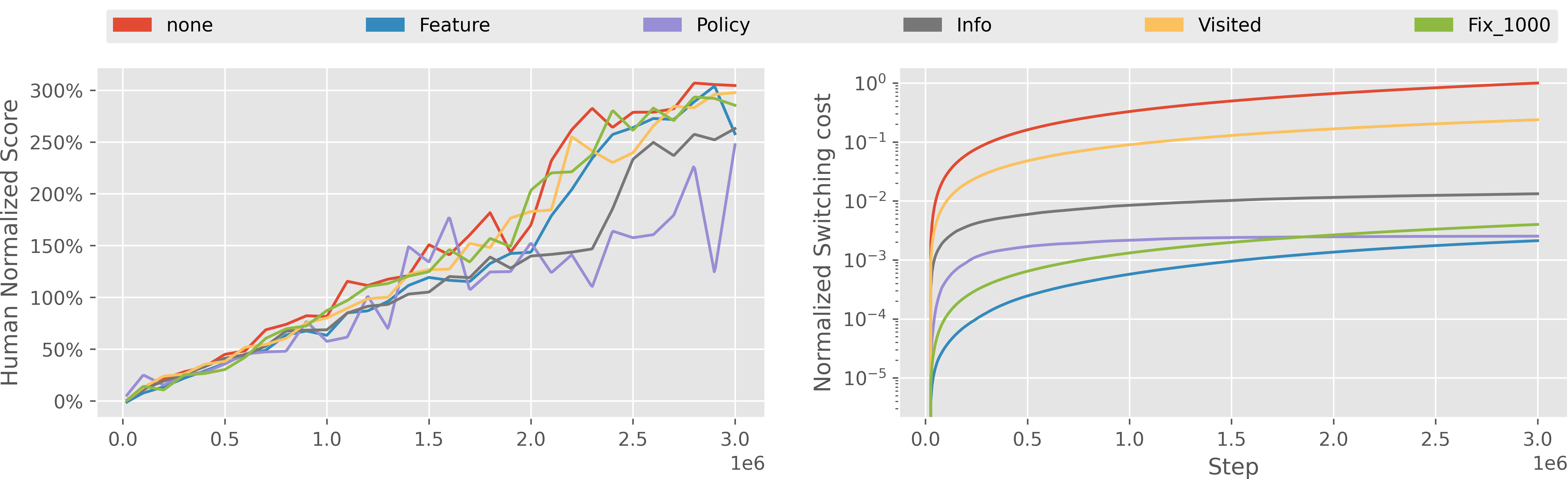
We then compare the performances of different switching criteria in the more complex Atari games. The state spaces in Atari games are images, which are more complicated than the low-dimensional states in GYMIC. Fig. 3 shows the average reward and switching of different switching criteria across all the 56 games, where the feature-based solution leads to the best empirical performance. We also remark that the non-adaptive baseline is particularly competitive in Atari games and outperforms all other adaptive solutions except the feature-based one. We also show the results in 8 representative games in Fig. 4, including the reward curves (odd rows) and switching cost curves (even rows). We can observe that information-gain variants produce substantially more policy updates while the feature-based and non-adaptive solutions are more stable.
In addition, we also noticed that the policy-based solution is particularly sensitive to its hyper-parameter in order to produce desirable policy reward, which suggests that the neural network features may change much more smoothly than the output action distribution.
To validate this hypothesis, we visualize the action difference and feature difference of the unconstrained Rainbow DQN on the Atari game “Pong” throughout the training process in Fig. 2. Note that in this case, the deployed policy is synced with the online policy in every training iteration, so the difference is merely due to a single training update. However, even in a unconstrained setting, the difference of action distribution fluctuates significantly. By contrast, the feature change is much more stable. We also provide some theoretical discussions on feature-based criterion in Appendix D.

MuJoCo Control:
We evaluate the effectiveness of different switching criteria with SAC on all the 6 MuJoCo continuous control tasks. The results are shown in Fig. 5. In general, we can still observe that the feature-based solution achieves the lowest switching cost among all the baseline methods while the policy-based solution produces the most unstable training. Interestingly, although the non-adaptive baseline has a relatively high switching cost than the feature-based one, the training curve has the less training fluctuations, which also suggests a future research direction on incorporating training stability into the switching criterion design.

| Avg. RSI | Feature | Policy | Info | Visitation | FIX_1000 |
|---|---|---|---|---|---|
| GYMIC | 9.63 | 4.16 | 8.88 | 0.0 | 6.91 |
| Atari | 3.61 | 2.82 | 2.11 | 1.81 | 3.15 |
| Mujoco | 8.20 | 3.45 | 4.83 | 1.92 | 6.91 |
Average RSI Scores: Finally, we also report the RSI scores of different policy switching criteria on different domains. For each domain, we compute the average value of RSI scores over each individual task in this domain. The results are reported in Table 1, where we can observe that the feature-based method consistently produces the best quantitative performance across all the 3 domains. 666We list the results of in Talbe 1, and also evaluate RSI using other . See appendix C for details.
In addition, we apply a -test for the switching costs among different criteria. The testing procedure is carried out for each pair of methods over all the experiment trials across all the environments and seeds. For Atari and MuJoCo, the results show that there are significant differences in switching cost between any two criteria (with -value < 0.05). For GYMIC, “None” and “Visited” is the only pair with no significant difference. It is also worth mentioning that RSI for “Visitation” for GYMIC is 0, which also shows the switching costs of “Visitation” and “None” are nearly the same.
6 Conclusion
In this paper, we focus on low-switching-cost reinforcement learning problems and take the first empirical step towards designing an effective solution for reducing the switching cost while maintaining good performance. By systematic empirical studies on practical benchmark environments with modern RL algorithms, we find the existence of a theory-practice gap in policy switching criteria and suggest a feature-based solution can be preferred in practical scenarios.
We remark that most theoretical works focus on simplified bandits or tabular MDPs when analysing mathematical properties of information-gain-based methods, but these theoretical insights are carried out on much simplified scenarios compared with popular deep RL testbeds that we consider here. In addition, these theoretical analyses often ignore the constant factors, which can be crucial for the practical use. By contrast, feature-based methods are much harder to analyze theoretically particularly in the use of non-linear approximators, which, however, produces much better practical performances. This also raises a new research direction for theoretical studies. We emphasize that our paper not only provides a benchmark but also raises many interesting open questions for algorithm development. For example, although feature-based solution achieves the best overall performance, it does not substantially outperform the the naive non-adaptive baseline. It still has a great research room towards designing a more principled switching criteria. Another direction is to give provable guarantees for these policy switching criteria that work for methods dealing with large state space in contrast to existing analyses about tabular RL [4, 27, 26]. We believe our paper is just the first step on this important problem, which could serve as a foundation towards great future research advances.
Thanks to the strong research nature of this work, we believe our paper does not produce any negative societal impact.
References
- [1] Yasin Abbasi-Yadkori, Dávid Pál, and Csaba Szepesvári. Improved algorithms for linear stochastic bandits. In John Shawe-Taylor, Richard S. Zemel, Peter L. Bartlett, Fernando C. N. Pereira, and Kilian Q. Weinberger, editors, Advances in Neural Information Processing Systems 24: 25th Annual Conference on Neural Information Processing Systems 2011. Proceedings of a meeting held 12-14 December 2011, Granada, Spain, pages 2312–2320, 2011.
- [2] Daniel Almirall, Scott N Compton, Meredith Gunlicks-Stoessel, Naihua Duan, and Susan A Murphy. Designing a pilot sequential multiple assignment randomized trial for developing an adaptive treatment strategy. Statistics in medicine, 31(17):1887–1902, 2012.
- [3] Peter Auer, Nicolo Cesa-Bianchi, and Paul Fischer. Finite-time analysis of the multiarmed bandit problem. Machine learning, 47(2-3):235–256, 2002.
- [4] Yu Bai, Tengyang Xie, Nan Jiang, and Yu-Xiang Wang. Provably efficient q-learning with low switching cost. In Advances in Neural Information Processing Systems, pages 8002–8011, 2019.
- [5] Nicolo Cesa-Bianchi, Ofer Dekel, and Ohad Shamir. Online learning with switching costs and other adaptive adversaries. In Advances in Neural Information Processing Systems, pages 1160–1168, 2013.
- [6] Minbo Gao, Tianle Xie, Simon S Du, and Lin F Yang. A provably efficient algorithm for linear markov decision process with low switching cost. arXiv preprint arXiv:2101.00494, 2021.
- [7] Shixiang Gu, Ethan Holly, Timothy Lillicrap, and Sergey Levine. Deep reinforcement learning for robotic manipulation with asynchronous off-policy updates. In 2017 IEEE international conference on robotics and automation (ICRA), pages 3389–3396. IEEE, 2017.
- [8] Tuomas Haarnoja, Aurick Zhou, Pieter Abbeel, and Sergey Levine. Soft actor-critic: Off-policy maximum entropy deep reinforcement learning with a stochastic actor. In International Conference on Machine Learning, pages 1861–1870. PMLR, 2018.
- [9] Matteo Hessel, Joseph Modayil, Hado van Hasselt, Tom Schaul, Georg Ostrovski, Will Dabney, Dan Horgan, Bilal Piot, Mohammad Gheshlaghi Azar, and David Silver. Rainbow: Combining improvements in deep reinforcement learning. In AAAI, 2018.
- [10] Han Hu, Kaicheng Zhang, Aaron Hao Tan, Michael Ruan, Christopher Agia, and Goldie Nejat. A sim-to-real pipeline for deep reinforcement learning for autonomous robot navigation in cluttered rough terrain. IEEE Robotics and Automation Letters, 6(4):6569–6576, 2021.
- [11] Natasha Jaques, Asma Ghandeharioun, Judy Hanwen Shen, Craig Ferguson, Agata Lapedriza, Noah Jones, Shixiang Gu, and Rosalind Picard. Way off-policy batch deep reinforcement learning of implicit human preferences in dialog. arXiv preprint arXiv:1907.00456, 2019.
- [12] Dmitry Kalashnikov, Jacob Varley, Yevgen Chebotar, Benjamin Swanson, Rico Jonschkowski, Chelsea Finn, Sergey Levine, and Karol Hausman. Mt-opt: Continuous multi-task robotic reinforcement learning at scale. CoRR, abs/2104.08212, 2021.
- [13] Aviral Kumar, Aurick Zhou, George Tucker, and Sergey Levine. Conservative q-learning for offline reinforcement learning. arXiv preprint arXiv:2006.04779, 2020.
- [14] Sascha Lange, Thomas Gabel, and Martin Riedmiller. Batch reinforcement learning. In Reinforcement learning, pages 45–73. Springer, 2012.
- [15] Sergey Levine, Aviral Kumar, George Tucker, and Justin Fu. Offline reinforcement learning: Tutorial, review, and perspectives on open problems. arXiv preprint arXiv:2005.01643, 2020.
- [16] Mufti Mahmud, M. Shamim Kaiser, Amir Hussain, and Stefano Vassanelli. Applications of deep learning and reinforcement learning to biological data. IEEE Trans. Neural Networks Learn. Syst., 29(6):2063–2079, 2018.
- [17] Travis Mandel, Yun-En Liu, Sergey Levine, Emma Brunskill, and Zoran Popovic. Offline policy evaluation across representations with applications to educational games. In AAMAS, pages 1077–1084, 2014.
- [18] Tatsuya Matsushima, Hiroki Furuta, Yutaka Matsuo, Ofir Nachum, and Shixiang Gu. Deployment-efficient reinforcement learning via model-based offline optimization. In International Conference on Learning Representations, 2021.
- [19] Azalia Mirhoseini, Anna Goldie, Mustafa Yazgan, Joe Jiang, Ebrahim M. Songhori, Shen Wang, Young-Joon Lee, Eric Johnson, Omkar Pathak, Sungmin Bae, Azade Nazi, Jiwoo Pak, Andy Tong, Kavya Srinivasa, William Hang, Emre Tuncer, Anand Babu, Quoc V. Le, James Laudon, Richard C. Ho, Roger Carpenter, and Jeff Dean. Chip placement with deep reinforcement learning. CoRR, abs/2004.10746, 2020.
- [20] Azalia Mirhoseini, Hieu Pham, Quoc V. Le, Benoit Steiner, Rasmus Larsen, Yuefeng Zhou, Naveen Kumar, Mohammad Norouzi, Samy Bengio, and Jeff Dean. Device placement optimization with reinforcement learning. In Doina Precup and Yee Whye Teh, editors, Proceedings of the 34th International Conference on Machine Learning, ICML 2017, Sydney, NSW, Australia, 6-11 August 2017, volume 70 of Proceedings of Machine Learning Research, pages 2430–2439. PMLR, 2017.
- [21] V. Mnih, K. Kavukcuoglu, D. Silver, Andrei A. Rusu, J. Veness, Marc G. Bellemare, A. Graves, Martin A. Riedmiller, Andreas K. Fidjeland, Georg Ostrovski, S. Petersen, C. Beattie, A. Sadik, Ioannis Antonoglou, H. King, D. Kumaran, Daan Wierstra, S. Legg, and Demis Hassabis. Human-level control through deep reinforcement learning. Nature, 518:529–533, 2015.
- [22] Yufei Ruan, Jiaqi Yang, and Yuan Zhou. Linear bandits with limited adaptivity and learning distributional optimal design. arXiv preprint arXiv:2007.01980, 2020.
- [23] Satinder P Singh, Tommi Jaakkola, and Michael I Jordan. Reinforcement learning with soft state aggregation. In Advances in neural information processing systems, pages 361–368, 1995.
- [24] Haoran Tang, Rein Houthooft, Davis Foote, Adam Stooke, Xi Chen, Yan Duan, John Schulman, F. Turck, and P. Abbeel. Exploration: A study of count-based exploration for deep reinforcement learning. ArXiv, abs/1611.04717, 2017.
- [25] Emanuel Todorov, Tom Erez, and Yuval Tassa. Mujoco: A physics engine for model-based control. In 2012 IEEE/RSJ International Conference on Intelligent Robots and Systems, pages 5026–5033, 2012.
- [26] Zihan Zhang, Xiangyang Ji, and Simon S. Du. Is reinforcement learning more difficult than bandits? a near-optimal algorithm escaping the curse of horizon. arXiv preprint arXiv:2009.13503, 2020.
- [27] Zihan Zhang, Yuan Zhou, and Xiangyang Ji. Almost optimal model-free reinforcement learning via reference-advantage decomposition, 2020.
- [28] Guanjie Zheng, Fuzheng Zhang, Zihan Zheng, Yang Xiang, Nicholas Jing Yuan, Xing Xie, and Zhenhui Li. DRN: A deep reinforcement learning framework for news recommendation. In Pierre-Antoine Champin, Fabien Gandon, Mounia Lalmas, and Panagiotis G. Ipeirotis, editors, Proceedings of the 2018 World Wide Web Conference on World Wide Web, WWW 2018, Lyon, France, April 23-27, 2018, pages 167–176. ACM, 2018.
| Supplementary Materials |
Appendix A Project Statement
Project website: https://sites.google.com/view/low-switching-cost-rl.
All of our code and detailed results can be found at our project website, including installation and running instructions for reproduciblity, and the results of individual games in Atari. The code is hosted at GitHub under the MIT license.
All the environments are public accessible RL testbeds. For experiments with MuJoCo engine, we register a free student license. All experiments are run on machines with 128 CPU cores, 256G memory, and one GTX 2080 GPU card.
Appendix B Experiment Details
B.1 Environments
GYMIC
GYMIC is an OpenAI gym environment for simulating sepsis treatment for ICU patients to an infection, where sepsis is caused by the body’s response to an infection and could be life-threatening. GYMIC built an environment to simulate the MIMIC sepsis cohort, where MIMIC is an open patient EHR dataset from ICU patients. This environment generates a sparse reward, the reward is set to +15 if the patient recovered and -15 if the patient died. This environment has 46 clinical features and a action space.
Atari 2600
Atari 2600 games are widely employed to evaluate the performance of DQN based agents. We evaluate the efficiency among different switching criteria on 56 games.
MuJoCo
MuJoCo contains continuous control tasks running in a physics simulator, we evaluate different switching criteria on 6 locomotion benchmarks.
For GYMIC and Atari games whose action space is discrete, we adopt Rainbow DQN to train the policy, for MuJoCo tasks with continuous action spaces, we employ SAC since it is more suitable for continuous action space.
B.2 Hyper-parameters of deterministic Rainbow
Table 2 lists the basic hyper-parameters of Rainbow. All of our experiments share these hyper-parameters except that the experiments on GYMIC adopt . Most of these hyper-parameters are the same as those in the original Rainbow algorithm. For count-based exploration, the bonus is set to 0.01.
| Parameter | Value |
|---|---|
| 20K | |
| learning rate | 0.0000625 |
| (Atari) | 8K |
| (GYMIC) | 1K |
| Adam | |
| Prioritization type | proportional |
| Prioritization exponent | 0.5 |
| Prioritization importance sampling | |
| Multi-step returns n | 3 |
| Distributional atoms | 51 |
| Distributional | [-10, 10] |
| Discount factor | 0.99 |
| Memory capacity N | 1M |
| Replay period | 4 |
| Minibatch size | 32 |
| Reward clipping | [-1, 1] |
| Count-base bonus | 0.01 |
| Activation function | ReLU |
Table 3 lists the extra hyper-parameters for experiments on GYMIC. Since there are 46 clinical features in this environment, we stack 4 consecutive states to compose a 184-dimensional vector as the input for the state encoder. The state encoder is a 2-layer MLP with hidden size 128.
| Parameter | Value |
|---|---|
| State Stacked | 4 |
| Number of layers for MLP | 2 |
| Hidden size | 128 |
Table 4 shows the additional hyper-parameters for experiments on Atari games. The observations are grey-scaled and resized to tensors with size , and 4 consecutive frames are concatenated as a single state. Each action selected by the agent is repeated for 4 times. The state encoder is composed of 3 convolutional layers with 32, 64 and 64 channels, which use 8x8, 4x4, 3x3 filters and strides of 4, 2, 1, respectively.
| Parameter | Value |
|---|---|
| Gray scaling | True |
| Observation | (84, 84) |
| Frame Stacked | 4 |
| Action repetitions | 4 |
| Max frames per episode | 108k |
| Encoder channels | 32, 64, 64 |
| Encoder filter size | |
| Encoder stride | 4, 2, 1 |
B.3 Hyper-parameters of SAC
We list the hyper-parameters of SAC in Table 5. We adopt Adam as the optimizer, the learning rate is set to 0.001 for MuJoCo control tasks except for Swimmer which is 0.0003, and the temperature parameter is set to 0.2 for Mujoco control tasks except for Humanoid which is 0.05. Other hyper-parameters are the same for these tasks. The update frequency “50/50” means we perform 50 iterations to update the online policy per 50 environment steps.
| Parameter | Value |
|---|---|
| Warm-up samples before training starts | 10K |
| Learning rate | 0.001 (0.0003 for Swimmer) |
| Optimizer | Adam |
| Temperature parameter | 0.2 (0.05 for Humanoid) |
| Discount factor | 0.99 |
| Memory capacity N | 1M |
| Number of hidden layers | 2 |
| Number of hidden nodes per layer | 256 |
| Target smoothing coefficient | 0.005 |
| Update frequency | 50/50 |
| Target update interval | 1 |
| Minibatch size | 128 |
| Activation function | ReLU |
B.4 Hyper-parameters of different criteria
For the switching threshold in policy-based and feature-based criteria (i.e., the mismatch ratio in policy-based criterion and parameter in feature-based criterion), we perform a rough grid search and choose the highest possible threshold that still produces a comparable final policy reward. For GYMIC, we tried and and finally adopted and . For Atari games, we tried and . For MuJoCo, we tried 777 is the thresholds of KL. and
Appendix C Discussion on RSI
C.1 RSI without log function
We choose log function because we observe that switching costs of different criteria vary in orders of magnitudes. We also tried a variant of RSI that removes the log function, which is
| (8) |
The results are shown in the following Table 6 ( = 0.2 ). We think these numbers have exaggerated the differences among different criteria and we finally adopt the log function.
| Feature | Policy | Info | Visitation | Fix_1000 | |
|---|---|---|---|---|---|
| MYGIC | 15152 | 64 | 7210 | 1 | 1000 |
| Atari | 1214 | 154 | 98 | 76 | 571 |
| MuJoCo | 10516 | 133 | 139 | 10 | 1000 |
C.2 Evaluate RSI with different
we evaluate RSI using different , and list the results in Table 7. Since the rewards obtained by different criteria on GYMIC are almost the same, RSI remains mostly unchanged when using different . The only exception is when . In this case, RSI of “Feature” and “Info” become 0. This is because a positive RSI requires strictly better or equal reward performance than “None” criterion when = 0. For Atari and MuJoCo, the overall trend is that a larger results in a larger RSI, since a larger tolerates a wider performance range. And we can observe that for most , the conclusions remain unchanged.
| MYGIC | ||||||||||
|---|---|---|---|---|---|---|---|---|---|---|
| 0.0 | 0.1 | 0.2 | 0.3 | 0.4 | 0.5 | 0.6 | 0.7 | 0.8 | 0.9 | |
| Feature | 0.0 | 9.63 | 9.63 | 9.63 | 9.63 | 9.63 | 9.63 | 9.63 | 9.63 | 9.63 |
| Policy | 4.16 | 4.16 | 4.16 | 4.16 | 4.16 | 4.16 | 4.16 | 4.16 | 4.16 | 4.16 |
| Info | 0.0 | 8.88 | 8.88 | 8.88 | 8.88 | 8.88 | 8.88 | 8.88 | 8.88 | 8.88 |
| Visitation | 0.0 | 0.0 | 0.0 | 0.0 | 0.0 | 0.0 | 0.0 | 0.0 | 0.0 | 0.0 |
| FIX_1000 | 6.91 | 6.91 | 6.91 | 6.91 | 6.91 | 6.91 | 6.91 | 6.91 | 6.91 | 6.91 |
| Atari | ||||||||||
| 0.0 | 0.1 | 0.2 | 0.3 | 0.4 | 0.5 | 0.6 | 0.7 | 0.8 | 0.9 | |
| Feature | 1.66 | 2.83 | 3.61 | 3.85 | 4.03 | 4.66 | 5.0 | 5.2 | 5.49 | 5.49 |
| Policy | 1.56 | 2.22 | 2.82 | 3.56 | 4.04 | 4.39 | 4.61 | 4.78 | 4.78 | 4.78 |
| Info | 0.81 | 1.46 | 2.11 | 2.89 | 3.23 | 3.66 | 4.19 | 4.27 | 4.35 | 4.35 |
| Visitation | 1.09 | 1.48 | 1.81 | 1.96 | 2.19 | 2.21 | 2.21 | 2.28 | 2.28 | 2.28 |
| FIX_1000 | 2.27 | 2.76 | 3.15 | 3.84 | 4.34 | 4.63 | 4.93 | 5.03 | 5.03 | 5.03 |
| MuJoCO | ||||||||||
| 0.0 | 0.1 | 0.2 | 0.3 | 0.4 | 0.5 | 0.6 | 0.7 | 0.8 | 0.9 | |
| Feature | 2.44 | 6.54 | 8.20 | 8.20 | 8.20 | 8.20 | 8.20 | 8.20 | 8.20 | 8.20 |
| Policy | 1.76 | 3.45 | 3.45 | 4.38 | 6.35 | 6.35 | 6.35 | 6.35 | 6.35 | 6.35 |
| Info | 2.40 | 4.83 | 4.83 | 4.83 | 4.83 | 4.83 | 4.83 | 4.83 | 4.83 | 4.83 |
| Visitation | 0.35 | 1.92 | 1.92 | 1.92 | 1.92 | 1.92 | 1.92 | 1.92 | 1.92 | 1.92 |
| FIX_1000 | 3.45 | 6.91 | 6.91 | 6.91 | 6.91 | 6.91 | 6.91 | 6.91 | 6.91 | 6.91 |
Appendix D Discussion on Feature-based Criterion
The feature-based criterion can be intuitively justified using some recent advances in representation learning theory. To illustrate the insight, we consider the following setting. Suppose we want to learn , a representation function that maps the input to a -dimension vector. We assume we have input-output pairs with for some underlying representation function and a linear predictor . For ease of presentation, let us assume we know , and our goal is to learn the underlying representation which together with gives us prediction error.
Suppose we have data sets and . We use to train an estimator of , denoted as , and to train another estimator of , denoted as The training method is empirical risk minimization, i.e.,
where is some pre-specified representation function class.
The following theorem suggests if the similarity score between and is small, then is also far from the underlying representation .
Theorem 1.
Suppose and are trained via aforementioned scheme. There exist dataset , , function class and such that if the similarity score between and on is smaller than , then the prediction error of on is .
Theorem 1 suggests that in certain scenarios, if the learned representation has not converged (the similarity score is small), then it cannot be the optimal representation which in turn will hurt the prediction accuracy. Therefore, if the similarity score is small, we should change the deployed policy.
Proof of Theorem 1.
We let be a -dimensional all one vector. We let
with being the ReLU activation function888We define and where denotes the vector that only the -th coordinate is and others are . We assume is an even number and is an integer for simplicity. We let the underlying be the vector correspond to . We let and . Because we use the ERM training scheme, it is clear that the training on will recover , i.e., because if it is not is better solution ( has error ) for the empirical risk. Now if the similarity score between and is smaller than , it means for , its corresponding are not correct. In this case, ’s prediction error is at least on , because it will predict on all inputs of .
∎