A Bayesian framework for patient-level partitioned survival cost-utility analysis

One important aspect, particularly in cancer trials, is that survival time can change rapidly after the disease has progressed. Therefore, inferences about mean utilities should take into account the specific features of pre- and post-progression responses as well as their dependence relationships. This is the rationale behind partitioned survival analysis, which involves the partitioning of survival data for the time to event end point, typically Overall Survival (OS), into two components: Progression Free Survival (PFS) and Post-Progression Survival (PPS), where $\text{OS}=\text{PFS}+\text{PPS}$. Hence, QAS based on the AUC approach can alternatively be computed during the pre- and post-progression periods by multiplying each survival component by the pre- and post-progression utilities. The partitioning of health-related quality of life data based on different components of survival time forms the basis for what is known as Partitioned Survival Cost-Utility Analysis, where patient-level QAS based on OS data ($\text{QAS}_{it}^{\text{OS}}$) can be expressed as

$$\text{QAS}^{\text{OS}}_{it}=\text{QAS}^{\text{PFS}}_{it}+\text{QAS}^{\text{PPS}}_{it},$$

(3)

where $\text{QAS}^{\text{PFS}}_{it}$ and $\text{QAS}^{\text{PPS}}_{it}$ are the QAS computed as in Equation 2 using patient-level utilities and survival times for pre- and post-progression periods, respectively. In most analyses, the different survival components in Equation 3 are separately modelled using parametric regression models to allow for extrapolation ^{6, 8}. However, in many cancer trials, direct modelling of $\text{QAS}^{\text{PPS}}_{it}$ is not possible since utility data are collected only up to progression, while utilities after disease progressions are extrapolated based on some modelling assumptions and OS or PFS data ⁹. However, if PPS is collected, it is generally recommended to use whatever of these data are available to improve the estimate of $\text{QAS}^{\text{PPS}}_{it}$.

It is important to note that the calculation of QAS in Equation 2 and Equation 3 assumes an absence of censoring. In practice, however, some of the patients may be still alive at the end of the trial (censored), which may hinder the validity of standard approaches for calculating QAS data. Indeed, on a QALY scale, survival times may be altered (by the utility weights), resulting in informative censoring (i.e. related to survival time), which makes the standard Kaplan-Meier analysis invalid ⁷. For the rest of the paper and in the analysis of our case study, we will assume that no informative censoring occurs (in the case study $>99\%$ of patients had died at the time of the analysis) so that standard partitioned survival cost-utility analysis methods for computing QAS data can be assumed to be valid. In Section 6 we will discuss the potential implications associated with informative censoring on these types of analyses as well as some alternative approaches that can be used to overcome the limitations associated with standard approaches in this context.

Statistical modelling for trial-based cost-effectiveness/utility data has received much attention in both the health economics and the statistical literature in recent years ^{10, 11}, increasingly often under a Bayesian statistical approach ^{12, 13, 14}. From the statistical point of view, this is a challenging problem because of the generally complex relationships linking the measure of effectiveness (e.g. QALYs) and the associated costs. First, the presence of a bivariate outcome requires the use of appropriate methods taking into account correlation ^{15, 16, 17}. Second, both utility and cost data are characterised by empirical distributions that are highly skewed and simplifying assumptions, such as (bivariate) normality of the underlying distributions, are usually not granted. The adoption of parametric distributions that can account for skewness (e.g. beta for the utilities and gamma or log-normal distributions for the costs) has been suggested to improve the fit of the model ^{18, 19, 20}. Third, data may exhibit spikes at one or both of the boundaries of the range for the underlying distribution, e.g. null costs and perfect health (i.e. utility of one), that are difficult to capture with standard parametric models ^{21, 20}. The use of more flexible formulations, known as hurdle models, has been recommended to explicitly account for these "structural" values ^{22, 23, 24}. These models consist in a mixture between a point mass distribution (the spike) and a parametric model fit to the natural range of the relevant variable without the boundary values. Finally, individual-level data from clinical trials are almost invariably affected by the problem of missing data. Analyses that are limited to individuals with fully-observed data (complete case analysis) are inefficient and assume that the completers are a random sample of all individuals, an assumption known as Missing Completely At Random (MCAR), which may yield biased inferences ²⁵. Alternative and more efficient approaches, such as multiple imputation and likelihood-based methods ^{25, 26}, rely on the less restrictive assumption that all observed data can be used to explain fully the reason for why some observations are missing, an assumption known as Missing At Random (MAR). However, the possibility that unobserved data influence the mechanism by which the missing values arise, an assumption known as Missing Not At Random (MNAR), can never be ruled out and will introduce bias when inferences are based on the observed data alone. Content-specific knowledge and tailored modelling approaches can be used to make inferences under MNAR and, within a Bayesian approach, informative prior distributions represent a powerful tool for conducting sensitivity analysis to different missingness assumptions ²⁷.

In this paper, we aim at extending the current methods for modelling trial-based partitioned survival cost-utility data, taking advantage of the flexibility of Bayesian methods, and specify a joint probabilistic model for the health economic outcomes. We propose a general framework that is able to account for the multiple types of complexities affecting individual level data (correlation, missingness, skewness and structural values), while also explicitly modelling the dependence relationships between different types of quality of life and cost components. The paper is structured as follows: first, in Section 2, we set out our modelling framework. In Section 3 we present the case study used as motivating example and describe the data, while Section 4 defines the general structure of the model used in the analysis and how it is tailored to deal with the different characteristics of the data. Section 5 presents and discusses the statistical and health economic results of the analysis. Finally, Section 6 summarises our conclusions.

For each individual and treatment, we specify a marginal distribution of the effectiveness variables $\bm{e}_{it}=(e^{\text{PFS}}_{it},e^{\text{PPS}}_{it})$ using the conditional factorisation:

$$p(\bm{e}_{it}\mid\bm{\theta}_{et})=p(e^{\text{PFS}}_{it}\mid\bm{\theta}^{\text{PFS}}_{et})p(e^{\text{PPS}}_{it}\mid e^{\text{PFS}}_{it},\bm{\theta}^{\text{PPS}}_{et}),$$

(5)

where $\bm{\theta}_{et}=(\bm{\theta}^{\text{PFS}}_{et},\bm{\theta}^{\text{PPS}}_{et})$ are the treatment-specific effectiveness parameters formed by the two distinct sets that index the marginal distribution of $e^{\text{PFS}}_{it}$ and the conditional distribution of $e^{\text{PPS}}_{it}\mid e^{\text{PFS}}_{it}$. The sets of parameters $\bm{\theta}_{et}$ can be expressed in terms of some location $\bm{\phi}_{iet}=(\phi^{\text{PFS}}_{iet},\phi^{\text{PPS}}_{iet})$ and ancillary $\bm{\psi}_{et}=(\bm{\psi}^{\text{PFS}}_{et},\bm{\psi}^{\text{PPS}}_{et})$ parameters, the latter typically comprising some standard deviations $\bm{\sigma}_{et}=(\sigma^{\text{PFS}}_{et},\sigma^{\text{PPS}}_{et})$. Often, interest is in the modelling of the location parameters as a function of other variables. This is typically achieved through a generalised linear structure and some link function that relates the expected value of the response to the linear predictors in the model. For example, we can use some parametric model to specify the distribution of the two effectiveness variables as

$$e^{\text{PFS}}_{it}\sim f^{\text{PFS}}(\phi^{\text{PFS}}_{iet},\bm{\psi}^{\text{PFS}}_{et})\;\;\;\text{and}\;\;\;e^{\text{PPS}}_{it}\mid e^{\text{PFS}}_{it}\sim f^{\text{PPS}}(\phi^{\text{PPS}}_{iet},\bm{\psi}^{\text{PPS}}_{et}),$$

(6)

where $f^{\text{PFS}}(\cdot)$ and $f^{\text{PPS}}(\cdot)$ denote some generic parametric distribution (e.g. normal) used to model $e^{\text{PFS}}_{it}$ and $e^{\text{PFS}}_{it}\mid e^{\text{PFS}}_{it}$, respectively. The locations of the two models in Equation 6 are then modelled as:

$$\begin{split}g(\phi^{\text{PFS}}_{iet})&=\alpha^{\text{PFS}}_{0t}+[\ldots],\\[7.74997pt] g(\phi^{\text{PPS}}_{iet})&=\alpha^{\text{PPS}}_{0t}+\alpha^{\text{PPS}}_{1t}(e^{\text{PFS}}_{it}-\mu^{\text{PFS}}_{et})+[\ldots],\end{split}$$

(7)

where $g(\cdot)$ is the link function, $\bm{\alpha}^{\text{PFS}}=(\alpha^{\text{PFS}}_{0t},\ldots)$ and $\bm{\alpha}^{\text{PPS}}=(\alpha^{\text{PPS}}_{0t},\alpha^{\text{PPS}}_{1t},\ldots)$ are the sets of regression parameters indexing the two models, while the notation $+\;[\ldots]$ indicates that other terms (e.g. quantifying the effect of relevant covariates $\bm{x}_{it}$) may or may not be included in each model. In the absence of covariates or assuming that a centred version $(\bm{x}_{it}-\bar{\bm{x}_{t}})$ is used, the quantities $\mu^{\text{PFS}}_{et}=g^{-1}(\alpha^{\text{PFS}}_{0})$ and $\mu^{\text{PPS}}_{et}=g^{-1}(\alpha^{\text{PPS}}_{0})$ can be interpreted as the population mean effectiveness for $e^{\text{PFS}}$ and $e^{\text{PPS}}$, respectively.

For the conditional distribution of the costs given the effectiveness, we use a similar approach to the one of $\bm{e}_{it}$ and factor $\bm{c}_{it}\mid\bm{e}_{it}$ as the product of a sequence of $K$ conditional distributions:

$$p(\bm{c}_{it}\mid\bm{e}_{it},\bm{\theta}_{ct})=p(c^{1}_{it}\mid\bm{e}_{it},\bm{\theta}^{1}_{ct})\cdot\cdot\cdot p(c^{K}_{it}\mid\bm{e}_{it},c^{1}_{it},\ldots,c^{K-1}_{it},\bm{\theta}^{K}_{ct}),$$

(8)

where $\bm{\theta}_{ct}=(\bm{\theta}^{1}_{ct},\ldots,\bm{\theta}^{K}_{ct})$ are the treatment-specific cost parameters that index the $K$ conditional distributions of the cost variables, with $K$ being the number of cost components. These parameters can also be expressed in terms of a series of $K$ location $\bm{\phi}_{ict}=(\phi^{1}_{ict},\ldots,\phi^{K}_{ict})$ and ancillary $\bm{\psi}_{ct}=(\psi^{1}_{ct},\ldots,\psi^{K}_{ct})$ parameters, the latter typically including a vector of standard deviations $\bm{\sigma}_{ct}=(\sigma^{1}_{ct},\ldots,\sigma^{K}_{ct})$. We can model the univariate distributions of the cost variables using some parametric forms:

$$c^{1}_{it}\mid\bm{e}_{it}\sim f^{1}(\phi^{1}_{ict},\bm{\psi}^{1}_{ct}),\;\;\;\cdot\cdot\cdot\,,\;\;\;c^{K}_{it}\mid\bm{e}_{it},c^{1}_{it},\ldots,c^{K-1}_{it}\sim f^{K}(\phi^{K}_{ict},\bm{\psi}^{K}_{ct}),$$

(9)

where $f^{1}(\cdot),\ldots,f^{K}(\cdot)$ denote the parametric distributions used to model the patient-level cost data for the $K$ cost components. The location of each variable can then be modelled as a function of other variables using the generalised linear forms:

$$\begin{split}g(\phi^{1}_{ict})&=\beta^{1}_{0t}+\beta^{1}_{1t}(e^{\text{PFS}}_{it}-\mu^{\text{PFS}}_{et})+\beta^{1}_{2t}(e^{\text{PPS}}_{it}-\mu^{\text{PPS}}_{et})+[\ldots],\\[7.74997pt] &\Large\vdots\\[7.74997pt] g(\phi^{K}_{ict})&=\beta^{K}_{0t}+\beta^{K}_{1t}(e^{\text{PFS}}_{it}-\mu^{\text{PFS}}_{et})+\beta^{K}_{2t}(e^{\text{PPS}}_{it}-\mu^{\text{PPS}}_{et})\;+\\[7.74997pt] &\quad\;\beta^{K}_{3t}(c^{1}_{it}-\mu^{1}_{ct})+\ldots+\beta^{K}_{K+1,t}(c^{K-1}_{it}-\mu^{K-1}_{ct})+[\ldots],\end{split}$$

(10)

where $\bm{\beta}^{1}=(\beta^{1}_{0t},\beta^{1}_{1t},\beta^{1}_{2t},\ldots),\ldots,\bm{\beta}^{K}=(\beta^{K}_{0t},\beta^{K}_{1t},\beta^{K}_{2t},\beta^{K}_{3t},\ldots,\beta^{K}_{K+1,t}\ldots)$ are the sets of regression parameters indexing the $K$ models. Assuming other covariates are also either centred or absent, the quantities $\mu^{1}_{ct}=g^{-1}(\beta^{1}_{0t}),\ldots,\mu^{K}_{ct}=g^{-1}(\beta^{K}_{0t})$ in Equation 10 can be interpreted as the $K$ population mean cost components.

Figure 1 provides a visual representation of the general modelling framework described above.

The effectiveness and cost distributions are represented in terms of combined "modules"- the red and blue boxes - in which the random quantities are linked through logical relationships. The links both within and between the variables in the modules ensure the full characterisation of the uncertainty in the model. Notably, this is general enough to be extended to any suitable distributional assumption, as well as to handle covariates in either or both the modules. In the following section, we first introduce and describe the case study that we use as motivating example. Next, we present the modelling specification for the effectiveness and cost data chosen in our analysis. The model is specified so to take into account different issues of the individual-level data, including correlation between variables, missingness, skewness and presence of structural values.

Throughout, we refer to our motivating example to demonstrate the flexibility of our approach in dealing with the different issues affecting the cost-utility data; we note that these are likely to be encountered in many practical cases, thus making our arguments applicable in general. We start by modelling $e^{\text{PFS}}_{it}$ with a Gumbel distribution using an identify link function for the mean:

$$\begin{split}e^{\text{PFS}}_{it}&\sim\text{Gumbel}(\phi^{\text{PFS}}_{et},\sigma^{\text{PFS}}_{et}),\\ \phi^{\text{PFS}}_{et}&=\alpha^{\text{PFS}}_{0t},\end{split}$$

(11)

where $\phi^{\text{PFS}}_{et}$ and $\sigma^{\text{PFS}}_{et}$ are the mean and standard deviation of $e^{\text{PFS}}_{it}$. We choose the Gumbel distribution since it was the parametric model associated with the best fit to the observed $e^{\text{PFS}}_{it}$ among those assessed (which included Logistic and Normal distributions). The Gumbel distribution has already been recommended for modelling utility data as it is defined on the real line while also being able to capture skewness ³¹.We parameterise the Gumbel distribution in terms of mean and standard deviation to facilitate the specification of the priors on the parameters, compared with using the canonical location $a$ (real) and scale $b>0$ parameters. More specifically, the mean and standard deviation of the Gumbel distribution are linked to the canonical parameters through the relationships: $a=\phi-b\kappa$ and $b=(\sigma\sqrt{6})/\pi$, where $\kappa$ is the Euler’s constant.

When choosing the model for $e^{\text{PPS}}_{it}$ it is important to take into account the considerable proportion of people associated with a zero value in the empirical distributions of both treatment groups (Figure 2), which may otherwise lead to biased inferences. We propose to handle this using a hurdle approach, where the distribution of $e^{\text{PPS}}_{it}$ is expressed as a mixture of a point mass distribution at zero and a parametric model for the natural range of the variable excluding the zeros. Specifically, for each subject we define an indicator variable $d^{PPS}_{it}$ taking value $1$ if the $i$-th individual is associated with $e^{\text{PPS}}_{it}=0$ and $0$ otherwise (i.e. $e^{\text{PFS}}_{it}>0$). We then model the conditional distribution of $d^{\text{PPS}}_{it}\mid e^{\text{PFS}}_{it}$ with a Bernoulli distribution using a logit link function for the probability of being associated with a zero:

$$\begin{split}d^{\text{PPS}}_{it}\mid e^{\text{PFS}}_{it}&\sim\text{Bernoulli}(\pi^{\text{PPS}}_{iet}),\\ \text{logit}(\pi^{\text{PPS}}_{iet})&=\gamma^{\text{PFS}}_{0t}+\gamma^{\text{PPS}}_{1t}e^{\text{PFS}}_{it},\end{split}$$

(12)

where $\pi^{\text{PPS}}_{iet}$ is the probability associated with $e^{\text{PPS}}_{it}=0$, which is expressed as a linear function of $e^{\text{PFS}}_{it}$ on the logit scale via the intercept and slope regression parameters $\gamma^{\text{PPS}}_{0t}$ and $\gamma^{\text{PPS}}_{1t}$, respectively. Other covariates which are thought to be strongly associated with the chance of having a zero can also be included in the logistic regression to improve the estimation of the probability parameter. However, in our analysis, the inclusion of any of the baseline variables available in the trial did not lead to substantial changes in the inferences, while also not improving the fit of the model to the observed data compared with Equation 12. Therefore, we decided to remove these variables and keep the current specification for the model of $d^{\text{PPS}}_{it}$. We model $e^{\text{PPS}}_{it}\mid d^{\text{PPS}}_{it}=0,e^{\text{PFS}}_{it}$ with an Exponential distribution using a log link function for the conditional mean:

$$\begin{split}e^{\text{PPS}}_{it}\mid d^{\text{PPS}}_{it}=0,e^{\text{PFS}}_{it}&\sim\text{Exponential}(\phi^{\text{PPS}}_{iet}),\\ \log(\phi^{\text{PPS}}_{iet})&=\alpha^{\text{PPS}}_{0t}+\alpha^{\text{PPS}}_{1t}e^{\text{PFS}}_{it},\end{split}$$

(13)

where $\alpha^{\text{PFS}}_{0t}$ and $\alpha^{\text{PPS}}_{1t}$ are the intercept and slope mean regression parameters for $e^{\text{PPS}}_{it}>0$, defined on the log scale. Again, the choice of the Exponential distribution was made according to the fit to the observed $e^{\text{PPS}}_{it}$ after comparing alternative model specifications (including Weibull and Normal distributions). We note that the canonical rate parameter $r$ of the Exponential distribution can be retrieved from the mean parameter through the relationship: $r=\frac{1}{\phi}$.

Using a similar modelling structure to that of $e^{\text{PPS}}_{it}$, we specify the models for the conditional distributions of the cost variables $\bm{c}_{it}=(c^{\text{drug}}_{it},c^{\text{hos}}_{it},c^{\text{ae}}_{it})$. We use a hurdle approach to handle the "structural" zero components for each variable, and fit Lognormal distributions to the positive costs (chosen in light of the better fit to the observed data compared with Gamma distributions). For each modelled cost variable, we checked whether the inclusion of any of the available baseline covariates from the trial could lead to some model improvement in terms of fit to the observed data or parameter estimates. However, results from the different model specifications suggest that there is no substantial gain from including these variables, which were therefore removed. We model the conditional distribution of the zero drug cost indicators and drug cost variables given $\bm{e}_{it}$ as:

$$\begin{split}d^{\text{drug}}_{it}\mid\bm{e}_{it}&\sim\text{Bernoulli}(\pi^{\text{drug}}_{ict}),\\ \text{logit}(\pi^{\text{drug}}_{ict})&=\delta^{\text{drug}}_{0t}+\delta^{\text{drug}}_{1t}e^{\text{PFS}}_{it}+\delta^{\text{drug}}_{2t}e^{\text{PPS}}_{it},\\[3.87498pt] c^{\text{drug}}_{it}\mid d^{\text{drug}}_{it}=0,\bm{e}_{it}&\sim\text{Lognormal}(\phi^{\text{drug}}_{ict},\sigma^{\text{drug}}_{ct}),\\ \phi^{\text{drug}}_{ict}&=\beta^{\text{drug}}_{0t}+\beta^{\text{drug}}_{1t}e^{\text{PFS}}_{it}+\beta^{\text{drug}}_{2t}e^{\text{PPS}}_{it},\end{split}$$

(14)

where $\pi^{\text{drug}}_{ict}$ is the probability of having $c^{\text{drug}}_{it}=0$, while $\phi^{\text{drug}}_{ict}$ and $\sigma^{\text{drug}}_{ct}$ are the mean and standard deviation parameter for $c^{\text{drug}}_{it}>0$ on the log scale. The regression parameters $\bm{\delta}^{\text{drug}}=(\delta^{\text{drug}}_{0t},\delta^{\text{drug}}_{1t},\delta^{\text{drug}}_{2t})$ and $\bm{\beta}^{\text{drug}}=(\beta^{\text{drug}}_{0t},\beta^{\text{drug}}_{1t},\beta^{\text{drug}}_{2t})$ capture the dependence between drug costs and the effectiveness variables for the zero and non-zero components, respectively. The conditional distribution of the zero hospital cost indicators and hospital cost variables given $\bm{e}_{it}$ and $c^{\text{drug}}_{it}$ is specified as:

$$\begin{split}d^{\text{hos}}_{it}\mid\bm{e}_{it},c^{\text{drug}}_{it}&\sim\text{Bernoulli}(\pi^{\text{hos}}_{ict}),\\ \text{logit}(\pi^{\text{hos}}_{ict})&=\delta^{\text{hos}}_{0t}+\delta^{\text{hos}}_{1t}e^{\text{PFS}}_{it}+\delta^{\text{hos}}_{2t}e^{\text{PPS}}_{it}+\delta^{\text{hos}}_{3t}\log(c^{\text{drug}}_{it}),\\[3.87498pt] c^{\text{hos}}_{it}\mid d^{\text{hos}}_{it}=0,\bm{e}_{it},c^{\text{drug}}_{it}&\sim\text{Lognormal}(\phi^{\text{hos}}_{ict},\sigma^{\text{hos}}_{ct}),\\ \phi^{\text{hos}}_{ict}&=\beta^{\text{hos}}_{0t}+\beta^{\text{hos}}_{1t}e^{\text{PFS}}_{it}+\beta^{\text{hos}}_{2t}e^{\text{PPS}}_{it}+\beta^{\text{hos}}_{3t}\log(c^{\text{drug}}_{it}),\end{split}$$

(15)

where $\pi^{\text{hos}}_{ict}$ is the probability of having $c^{\text{hos}}_{it}=0$, while $\phi^{\text{hos}}_{ict}$ and $\sigma^{\text{hos}}_{ct}$ are the mean and standard deviation parameter for $c^{\text{hos}}_{it}>0$ on the log scale. The regression parameters $\bm{\delta}^{\text{hos}}$ and $\bm{\beta}^{\text{hos}}$ capture the dependence between hospital costs, the effectiveness and the drug cost variables for the zero and non-zero components, respectively. Finally, we specify the conditional distribution of the zero adverse event cost indicators and adverse events cost variables given $\bm{e}_{it}$, $c^{\text{drug}}_{it}$ and $c^{\text{hos}}_{it}$ as:

$$\begin{split}d^{\text{ae}}_{it}\mid\bm{e}_{it},c^{\text{drug}}_{it},c^{\text{hos}}_{it}&\sim\text{Bernoulli}(\pi^{\text{ae}}_{ict}),\\ \text{logit}(\pi^{\text{ae}}_{ict})&=\delta^{\text{ae}}_{0t}+\delta^{\text{ae}}_{1t}e^{\text{PFS}}_{it}+\delta^{\text{ae}}_{2t}e^{\text{PPS}}_{it}+\delta^{\text{ae}}_{3t}\log(c^{\text{drug}}_{it})+\delta^{\text{ae}}_{4t}\log(c^{\text{hos}}_{it}),\\[3.87498pt] c^{\text{ae}}_{it}\mid d^{\text{ae}}_{it}=0,\bm{e}_{it},c^{\text{drug}}_{it},c^{\text{hos}}_{it}&\sim\text{Lognormal}(\phi^{\text{ae}}_{ict},\sigma^{\text{ae}}_{ct}),\\ \phi^{\text{ae}}_{ict}&=\beta^{\text{ae}}_{0t}+\beta^{\text{ae}}_{1t}e^{\text{PFS}}_{it}+\beta^{\text{ae}}_{2t}e^{\text{PPS}}_{it}+\beta^{\text{ae}}_{3t}\log(c^{\text{drug}}_{it})+\beta^{\text{ae}}_{4t}\log(c^{\text{hos}}_{it}),\end{split}$$

(16)

where $\pi^{\text{ae}}_{ict}$ is the probability of having $c^{\text{ae}}_{it}=0$, while $\phi^{\text{ae}}_{ict}$ and $\sigma^{\text{ae}}_{ct}$ are the mean and standard deviation parameter for $c^{\text{ae}}_{it}>0$ on the log scale. The regression parameters $\bm{\delta}^{\text{ae}}$ and $\bm{\beta}^{\text{ae}}$ capture the dependence between adverse events costs, hospital costs, the effectiveness and the drug cost variables for the zero and non-zero components, respectively. We note that we included the drug and hospital cost variables on the log scale in both logit and log linear regressions in Equation 15 and Equation 16 as this lead to an improvement of the model fit compared with using the costs on the original scale. For all parameters in the model we specify vague prior distributions: a normal distribution with a large variance on the appropriate scale for the regression parameters, e.g. $\text{Normal}(0,10000)$, and a uniform distribution over a large positive range for the standard deviations, e.g. $\text{Uniform}(0,10000)$.

We note that, although the proposed model requires the specification of a relatively large number of parameters, which may make the model difficult to interpret, this, however, does not ultimately affect the final analysis, which exclusively focuses on the marginal effectiveness and cost means ($\mu_{et}$ and $\mu_{ct}$). These quantities can be retrieved by centering each variable in the effectiveness and cost modules as shown in Section 2. However, this procedure may become difficult to implement in practice when dealing with non-standard parametric specifications, such as the hurdle models, which make the identification of such parameters cumbersome. An alternative, although more computationally intensive, approach to overcome this problem is Monte Carlo integration, which allows to retrieve the marginal mean estimates for each variable by randomly drawing a large number of samples from the posterior distribution of the model and then take the expectation over these sampled values as an approximation to the marginal means.

The procedure is defined as follows. First, we fit the model to the full data, typically using some Markov Chain Monte Carlo (MCMC) methods ³² and imputing the missing values based on their predictive distributions conditional on the observed data via some data augmentation procedure ³³. Second, at each iteration of the posterior distribution, we generate a large number of samples for each component of $\bm{e}_{it}$ and $\bm{c}_{it}$ based on the posterior values for the parameters of the effectiveness and cost models in the MCMC output. Third, we approximate the posterior distribution of the marginal means by taking the expectation over the sampled values at each iteration. Finally, we derive the overall marginal means $\bm{\mu}=(\mu_{et},\mu_{ct})$ by summing up the marginal mean estimates for the different components of the effectiveness and costs, that is:

$$\mu_{et}=\mu^{\text{PFS}}_{et}+\mu^{\text{PPS}}_{et}\;\;\;\text{and}\;\;\;\mu_{ct}=\mu^{\text{drug}}_{ct}+\mu^{\text{hos}}_{ct}+\mu^{\text{ae}}_{ct},$$

(17)

where $\mu^{\text{PFS}}_{et}$ and $\mu^{\text{PPS}}_{et}$ are the pre- and post-progression mean QAS, while $\mu^{\text{drug}}_{ct}$, $\mu^{\text{hos}}_{ct}$ and $\mu^{\text{ae}}_{ct}$ are the mean for the three different components (drug, hospital and adverse events) in the TOPICAL trial.

We fitted the model in STAN ³⁴ which is a software specifically designed for the analysis of Bayesian models using a type of MCMC algorithm known as Hamiltonian Monte Carlo 32, and which is interfaced with R through the package rstan ³⁵. Samples from the posterior distribution of the parameters of interest generated by STAN and saved to the R work space are then used to produce summary statistics and plots. We ran two chains with $15000$ iterations per chain, using a burn-in of $3000$, for a total sample of $24000$ iterations for posterior inference. For each unknown quantity in the model, we assessed convergence and autocorrelation of the MCMC simulations by using diagnostic measures including density and trace plots, the potential scale reduction factor and the effective sample size ³⁶. A summary of the results from these convergence checks for the parameters of the model are provided in Appendix B, while the STAN code used to fit the model is provided in the supplementary material.

We compute two relative measures of predictive accuracy to assess the fit of the proposed model specification (denoted as "original") with respect to a second parametric specification (denoted as "alternative"), where we replace the Gumbel distribution for $e^{\text{PFS}}_{it}$ with a Logistic distribution, the Exponential distribution for $e^{\text{PPS}}_{it}>0$ with a Weibull distribution, and the Lognormal distributions for $\bm{c}_{it}>0$ with Gamma distributions. We specifically rely on the Widely Applicable Information Criterion (WAIC) ³⁷ and the Leave-One-Out Information Criterion (LOOIC) ³⁸, which provide estimates for the pointwise out-of-sample prediction accuracy from a fitted Bayesian model using the log-likelihood evaluated at the posterior simulations of the parameter values. Both measures can be viewed as an improvement on the popular Deviance Information Criterion (DIC) ³⁹ in that they use the entire posterior distribution, are invariant to parametrisation, and are asymptotically equal to Bayesian cross-validation ⁴⁰. These information criteria are obtained based on the model deviance and a penalty for model complexity known as effective number of parameters ($p_{D}$ ) and, when comparing a set of models based on the same data, the one associated with the lowest WAIC or LOOIC is the best-performing, among those assessed.

Results between the two alternative specifications are reported in Table 1.

For both criteria, the values associated with the "original" specification of the model are systematically lower compared with those from the "alternative" parameterisation, and result in an overall better fit to the data for the first model. We have explored different configurations of distribution assignment among those shown in Table 1 for the effectiveness and cost variables (including also the Normal distribution which, however, was always associated with the worst fit). The results from these comparisons suggest that the "original" specification of the model remains the one associated with the best performance.

We additionally assess the absolute fit of the model using the observed and replicated data. The latter are generated from the posterior predictive distributions of the models using the posterior samples of the parameters indexing the distributions of each effectiveness and cost variable. We use the posterior estimates from these parameters to jointly sample $10000$ replications of the data which are then used for model assessment. We computed different types of graphical posterior predictive checks, either in terms of the entire distributions using density and cumulative density plots, or in terms of the marginal mean estimates between the real and replicated data, which are provided in Appendix C. Overall these checks suggest a relatively good fit of the model for each modelled variable.

Figure 4 compares the posterior means (squares) together with the $50\%$ (thick lines) and $95\%$ (thin lines) highest posterior density (HPD) credible intervals for the marginal means of each effectiveness and cost components, obtained from fitting the model to all cases under a MAR assumption. Results associated with the control ($t=1$) and intervention ($t=2$) group are indicated with red and blue colours, respectively.

Posterior QAS means are on average higher for the PFS compared with the PPS component in both treatment groups. However, both $50\%$ and $95\%$ HPD intervals suggest that the estimates associated with the intervention group have a much higher degree of variability compared with those from the control, especially for the PPS component. The posterior cost means for each component show that the intervention group is associated with systematically higher values with respect to the control, especially for the drug costs which by far cover most of the total costs in the intervention. HPD intervals for mean costs show a relatively high degree of skewness with posterior mean estimates being closer to the upper bounds of the $50\%$ intervals compared to the lower bounds.

We derived the aggregated QAS and cost means for each treatment group $(\mu_{et},\mu_{ct})$ by summing up the posterior mean estimates of the different components for each type of variable. We then computed the incremental mean estimates between the two groups, denoted with $\Delta_{e}=\mu_{e2}-\mu_{e1}$ and $\Delta_{c}=\mu_{c2}-\mu_{c1}$, together with the Incremental Cost Effectiveness Ratio (ICER), representing the cost per QAS gained between the two interventions. Table 2 shows selected posterior summaries, including means, medians, standard deviations and $95\%$ HPD intervals, for the marginal and incremental mean estimates associated with the two intervention groups.

Overall, the posterior results indicate that the new intervention is associated with systematically higher QAS and costs compared to the control, with a positive mean QAS increment of $0.17$, a positive mean cost increment of $\pounds 12602$, and with $95\%$ intervals that exclude zero for both quantities. We note that posterior estimates for the marginal means in the control group show a considerably lower degree of variability (standard deviations of $0.02$ and $\pounds 424$) compared with those from the intervention group (standard deviations of $0.05$ and $\pounds 2628$). Finally, the additional cost per unit of QAS gained is estimated to be roughly $\pounds 80000$ for $t=2$ compared to $t=1$.

We complete the analysis by assessing the probability of cost-effectiveness for the new intervention with respect to the control. A general advantage of using a Bayesian approach is that the economic analysis can be easily performed without the need to use ad-hoc methods to represent uncertainty around point estimates (e.g. bootstrapping). Indeed, once the statistical model is fitted to the data, the samples from the posterior distributions of the parameters of interest can be used to compute different types of summary measures of cost-effectiveness.

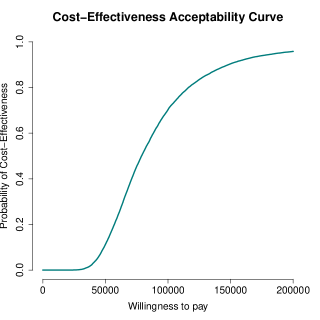
We specifically rely on the examination of the cost-effectiveness plane (CEP) ⁴¹ and the cost-effectiveness acceptability curve (CEAC) ⁴² to summarise the economic analysis. Figure 5 (panel a) shows the plot of the CEP, which is a graphical representation of the joint distribution for the mean effectiveness and costs increments between the two treatment groups. The slope of the straight line crossing the plane is the "willingness-to-pay’" threshold (which is often indicated as $k$). This can be considered as the amount of budget that the decision maker is willing to spend to increase the health outcome of $1$ unit and effectively is used to trade clinical benefits for money. Current recommendations for generic interventions suggest a value of $k$ between $\pounds 20000-30000$; however, for end of life treatments, such as cancer treatments, the recommended threshold values are typically higher and lie in a range between $\pounds 50000-60000$ or above ⁴³. Points lying below this straight line fall in the so-called sustainability area ¹⁴ and suggest that the new intervention is more cost-effective than the control.

Almost all samples fall in the north-east quadrant of the plane. This suggests that the intervention is likely to be more effective and more expensive compared with the control. At $k=\pounds 55000$, the ICER (and the majority of the samples) falls outside the sustainability area, and therefore indicates that the intervention is unlikely to be considered cost-effective at the chosen value of $k$. Figure 5 (panel b) shows the CEAC, which is obtained by computing the proportion of points lying in the sustainability area on varying the willingness-to-pay threshold $k$. The CEAC estimates the probability of cost-effectiveness, thus providing a simple summary of the uncertainty that is associated with the "optimal" decision making that is suggested by the ICER. The graph shows how, starting from null to relatively small probabilities of cost-effectiveness for $k<\pounds 50000$, as the value of the willingness to pay threshold is increased, the chance that the new intervention becomes cost-effective rises up to near full certainty for $k>\pounds 150000$. We note that these cost-effectiveness conclusions should be interpreted with care, due to limitations associated with the data analysed which are explicitly discussed in Section 6 (e.g. based on a subset of the original data). However, this does not affect the generalisability of our framework, which implements a flexible modelling approach for handling the typical characteristics of trial-based partitioned survival economic data.

References

- Earnshaw and Lewis 2008 Julia Earnshaw and Gavin Lewis. Nice guide to the methods of technology appraisal, 2008.
- Glick et al. 2014 Henry A Glick, Jalpa A Doshi, Seema S Sonnad, and Daniel Polsky. Economic evaluation in clinical trials. OUP Oxford, 2014.
- Van Reenen and Oppe 2015 M. Van Reenen and M. Oppe. EQ-5D-3L User Guide Basic information on how to use the EQ-5D-3L instrument. https://euroqol.org/wp-content/uploads/2016/09/EQ-5D-3L_UserGuide_2015.pdf, 2015.
- Dolan 1997 Paul Dolan. Modeling valuations for euroqol health states. Medical care, pages 1095–1108, 1997.
- Drummond et al. 2005 MF. Drummond, MJ. Schulpher, K. Claxton, GL. Stoddart, and GW. Torrance. Methods for the economic evaluation of health care programmes. 3rd ed. Oxford university press, Oxford, 2005.
- Khan 2015 Iftekhar Khan. Design & Analysis of clinical trials for Economic Evaluation & Reimbursement: an applied approach using SAS & STATA. Chapman and Hall/CRC, 2015.
- Glasziou et al. 1990 PP Glasziou, RJ Simes, and RD Gelber. Quality adjusted survival analysis. Statistics in medicine, 9(11):1259–1276, 1990.
- Gelber et al. 1995 Richard D Gelber, Bernard F Cole, Shari Gelber, and Aron Goldhirsch. Comparing treatments using quality-adjusted survival: the q-twist method. The American Statistician, 49(2):161–169, 1995.
- Williams et al. 2017 Claire Williams, James D Lewsey, Daniel F Mackay, and Andrew H Briggs. Estimation of survival probabilities for use in cost-effectiveness analyses: a comparison of a multi-state modeling survival analysis approach with partitioned survival and markov decision-analytic modeling. Medical Decision Making, 37(4):427–439, 2017.
- Willan and Briggs 2006 Andrew R Willan and Andrew H Briggs. Statistical analysis of cost-effectiveness data, volume 37. John Wiley & Sons, 2006.
- Ramsey et al. 2015 Scott D Ramsey, Richard J Willke, Henry Glick, Shelby D Reed, Federico Augustovski, Bengt Jonsson, Andrew Briggs, and Sean D Sullivan. Cost-effectiveness analysis alongside clinical trials ii—an ispor good research practices task force report. Value in Health, 18(2):161–172, 2015.
- O’Hagan et al. 2001 Anthony O’Hagan, John W Stevens, and Jacques Montmartin. Bayesian cost-effectiveness analysis from clinical trial data. Statistics in medicine, 20(5):733–753, 2001.
- Spiegelhalter et al. 2004 David J Spiegelhalter, Keith R Abrams, and Jonathan P Myles. Bayesian approaches to clinical trials and health-care evaluation, volume 13. John Wiley & Sons, 2004.
- Baio 2012 G. Baio. Bayesian Methods in Health Economics. Chapman and Hall/CRC, University College London London, UK, 2012.
- Nixon and Thompson 2005 RM. Nixon and SG. Thompson. Methods for incorporating covariate adjustment, subgroup analysis and between-centre differences into cost-effectiveness evaluations. Health Economics, 14:1217–1229, 2005.
- Grieve et al. 2010 R. Grieve, R. Nixon, G. Simon, and SG. Thompson. Bayesian hierarchical models for cost-effectiveness analyses that use data from cluster randomized trials. Medical Decision Making, 30:163–175, 2010.
- Gomes et al. 2012 R. Gomes, ESW. Ng, R. Grieve, R. Nixon, ESW. NG, J. Carpenter, and SG. Thompson. Developing appropriate methods for cost-effectiveness analysis of cluster randomized trials. Medical Decision Making, 32:350–361, 2012.
- O’Hagan and Stevens 2003 A. O’Hagan and JW. Stevens. Assessing and comparing costs: how robust are the bootstrap and methods based on asymptotic normality? Health Economics, 12:33–49, 2003.
- Thompson and Nixon 2005 SG. Thompson and RM. Nixon. How sensitive are cost-effectiveness analyses to choice of parametric distributions? Medical Decision Making, 4:416–423, 2005.
- Basu et al. 2007 A. Basu, JJ. Heckman, S. Navarro-Lozano, and S. Urzua. Use of instrumental variables in the presence of heterogeneity and self-selection: An application in breast cancer patients. Health Econometrics and Data Group, HEDG Working Paper 07/07, 2007.
- Mihaylova et al. 2011 Borislava Mihaylova, Andrew Briggs, Anthony O’Hagan, and Simon G Thompson. Review of statistical methods for analysing healthcare resources and costs. Health economics, 20(8):897–916, 2011.
- Baio 2014 Gianluca Baio. Bayesian models for cost-effectiveness analysis in the presence of structural zero costs. Statistics in medicine, 33(11):1900–1913, 2014.
- Gabrio et al. 2019a Andrea Gabrio, Alexina J Mason, and Gianluca Baio. A full bayesian model to handle structural ones and missingness in economic evaluations from individual-level data. Statistics in medicine, 38(8):1399–1420, 2019a.
- Gabrio et al. 2019b Andrea Gabrio, Michael J Daniels, and Gianluca Baio. A bayesian parametric approach to handle missing longitudinal outcome data in trial-based health economic evaluations. Journal of the Royal Statistical Society: Series A (Statistics in Society), 2019b.
- Rubin 1987 DB. Rubin. Multiple Imputation for Nonresponse in Surveys. John Wiley and Sons, New York,USA, 1987.
- Molenberghs et al. 2014 Geert Molenberghs, Garrett Fitzmaurice, Michael G Kenward, Anastasios Tsiatis, and Geert Verbeke. Handbook of missing data methodology. Chapman and Hall/CRC, 2014.
- Daniels and Hogan 2008 MJ. Daniels and JW. Hogan. Missing Data in Longitudinal Studies: Strategies for Bayesian Modeling and Sensitivity Analysis. Chapman and Hall, New York, 2008.
- Lambert et al. 2008 Paul C Lambert, Lucinda J Billingham, Nicola J Cooper, Alex J Sutton, and Keith R Abrams. Estimating the cost-effectiveness of an intervention in a clinical trial when partial cost information is available: a bayesian approach. Health economics, 17(1):67–81, 2008.
- Lee et al. 2012 Siow Ming Lee, Iftekhar Khan, Sunil Upadhyay, Conrad Lewanski, Stephen Falk, Geraldine Skailes, Ernie Marshall, Penella J Woll, Matthew Hatton, Rohit Lal, et al. First-line erlotinib in patients with advanced non-small-cell lung cancer unsuitable for chemotherapy (topical): a double-blind, placebo-controlled, phase 3 trial. The lancet oncology, 13(11):1161–1170, 2012.
- Khan et al. 2015 Iftekhar Khan, Stephen Morris, Allan Hackshaw, and Siow-Ming Lee. Cost-effectiveness of first-line erlotinib in patients with advanced non-small-cell lung cancer unsuitable for chemotherapy. BMJ open, 5(7):e006733, 2015.
- Gomes et al. 2019 Manuel Gomes, Rosalba Radice, Jose Camarena Brenes, and Giampiero Marra. Copula selection models for non-gaussian outcomes that are missing not at random. Statistics in medicine, 38(3):480–496, 2019.
- Brooks et al. 2011 Steve Brooks, Andrew Gelman, Galin Jones, and Xiao-Li Meng. Handbook of markov chain monte carlo. CRC press, 2011.
- Tanner and Wong 1987 Martin A Tanner and Wing Hung Wong. The calculation of posterior distributions by data augmentation. Journal of the American statistical Association, 82(398):528–540, 1987.
- Carpenter et al. 2017 Bob Carpenter, Andrew Gelman, Matthew D Hoffman, Daniel Lee, Ben Goodrich, Michael Betancourt, Marcus Brubaker, Jiqiang Guo, Peter Li, and Allen Riddell. Stan: A probabilistic programming language. Journal of statistical software, 76(1), 2017.
- Team et al. 2016 Stan Developent Team et al. Rstan: the r interface to stan. R package version, 2(1), 2016.
- Gelman et al. 2004 A. Gelman, J. Carlin, H. Stern, and D. Rubin. Bayesian Data Analysis - 2nd edition. Chapman and Hall, New York, NY, 2004.
- Watanabe 2010 Sumio Watanabe. Asymptotic equivalence of bayes cross validation and widely applicable information criterion in singular learning theory. Journal of Machine Learning Research, 11(Dec):3571–3594, 2010.
- Vehtari et al. 2017 Aki Vehtari, Andrew Gelman, and Jonah Gabry. Practical bayesian model evaluation using leave-one-out cross-validation and waic. Statistics and computing, 27(5):1413–1432, 2017.
- Spiegelhalter et al. 2002 David J Spiegelhalter, Nicola G Best, Bradley P Carlin, and Angelika Van Der Linde. Bayesian measures of model complexity and fit. Journal of the royal statistical society: Series b (statistical methodology), 64(4):583–639, 2002.
- Gelman et al. 2014 Andrew Gelman, Jessica Hwang, and Aki Vehtari. Understanding predictive information criteria for bayesian models. Statistics and computing, 24(6):997–1016, 2014.
- Black 1990 WC. Black. A graphic representation of cost-effectiveness. Medical Decision Making, 10:212–214, 1990.
- Van Hout et al. 1994 BA. Van Hout, MJ. Al, GS. Gordon, FFH. Rutten, and KM. Kuntz. Costs, effects and c/e-ratios alongside a clinical trial. Health Economics, 3:309–319, 1994.
- NICE 2013 NICE. Guide to the Methods of Technological Appraisal. NICE, London, 2013.
- O’Hagan and Stevens 2001 A. O’Hagan and JW. Stevens. A framework for cost-effectiveness analysis from clinical trial data. Health Economics, 10:303–315, 2001.
- Claxton 1999 Karl Claxton. The irrelevance of inference: a decision-making approach to the stochastic evaluation of health care technologies. Journal of health economics, 18(3):341–364, 1999.
- Claxton et al. 2005 K. Claxton, M. Sculpher, C. McCabe, A. Briggs, R. Hakehurst, M. Buxton, J. Brazier, and T. O’Hagan. Probabilistic sensitivity analysis for nice technology assessment: not an optional extra. Heath Economics, 27:339–347, 2005.
- Mason et al. 2018 Alexina J Mason, Manuel Gomes, Richard Grieve, and James R Carpenter. A bayesian framework for health economic evaluation in studies with missing data. Health economics, 27(11):1670–1683, 2018.
- Gabry and Mahr 2018 Jonah Gabry and T Mahr. bayesplot: Plotting for bayesian models. r package version 1.6. 0, 2018.
Appendix A Missingness Patterns in TOPICAL
TABLE 3
Appendix B MCMC Convergence
This section reports some summary diagnostics of the MCMC algorithm, including density and trace plots, for all key parameters of the model fitted to the TOPICAL data. For all parameters, no substantial issue in convergence is detected. All plots were generated from R using functions in the package bayesplot 48, which provides a variety of tools to perform diagnostic and posterior predictive checks for Bayesian models.
FIGURE 6
FIGURE 7
FIGURE 8
FIGURE 9
Appendix C Posterior Predictive Checks
This section reports some graphical posterior predictive checks, including empirical density, cumulative density and mean plots, for all variables of the model fitted to each treatment group in the TOPICAL trial. In all cases, no substantial discrepancy between the observed and predicted data is detected which suggests a generally good fit of the model. All plots were generated from R using functions in the package bayesplot 48, which provides a variety of tools to perform diagnostic and posterior predictive checks for Bayesian models.