4D Gaussian Splatting: Modeling Dynamic Scenes with Native 4D Primitives
Abstract
Dynamic 3D scene representation and novel view synthesis from captured videos are crucial for enabling immersive experiences required by AR/VR and metaverse applications. However, this task is challenging due to the complexity of unconstrained real-world scenes and their temporal dynamics. In this paper, we frame dynamic scenes as a spatio-temporal 4D volume learning problem, offering a native explicit reformulation with minimal assumptions about motion, which serves as a versatile dynamic scene learning framework. Specifically, we represent a target dynamic scene using a collection of 4D Gaussian primitives with explicit geometry and appearance features, dubbed as 4D Gaussian splatting (4DGS). This approach can capture relevant information in space and time by fitting the underlying spatio-temporal volume. Modeling the spacetime as a whole with 4D Gaussians parameterized by anisotropic ellipses that can rotate arbitrarily in space and time, our model can naturally learn view-dependent and time-evolved appearance with 4D spherindrical harmonics. Notably, our 4DGS model is the first solution that supports real-time rendering of high-resolution, photorealistic novel views for complex dynamic scenes. To enhance efficiency, we derive several compact variants that effectively reduce memory footprint and mitigate the risk of overfitting. Extensive experiments validate the superiority of 4DGS in terms of visual quality and efficiency across a range of dynamic scene-related tasks (e.g., novel view synthesis, 4D generation, scene understanding) and scenarios (e.g., single object, indoor scenes, driving environments, synthetic and real data).
Index Terms:
Dynamic scenes, novel view synthesis, Gaussian splatting, neural video synthesis.I Introduction
Modeling dynamic scenes from 2D images and rendering novel views in real-time is crucial in computer vision and graphics, which has received increasing attention from both industry and academia because of its potential value in a wide range of AR/VR applications. Whilst recent breakthroughs (e.g., NeRF [1]) have achieved photorealistic rendering for static scenes [2, 3], handling dynamic scenes remains a significant challenge. The temporal dynamics of scenes introduce additional complexity. The central challenge lies in preserving intrinsic correlations and sharing relevant information across different time steps, all while minimizing interference between unrelated spacetime locations.

Existing novel view synthesis methods for dynamic scenes can be categorized into two groups. The first group directly learns parametric 6D plenoptic functions using implicit neural models, employing structures such as MLPs [4], grids [5], or their low-rank decompositions [6, 7, 8], without explicitly modeling scene motion. Their ability to capture correlations across varying spatiotemporal locations relies on the intrinsic properties of the selected data structure. As a result, these methods may experience interference due to shared parameters across spatiotemporal locations or struggle to leverage the inherent correlations arising from object motion effectively.
The second group posits that scene dynamics underlie the motion and deformation of a single 3D model [9, 10, 11, 12]. These approaches explicitly model scene motion, potentially improving the utilization of spatial and temporal correlations. However, global tracking of object motion involves inherent ambiguities and risks singularities when dealing with complex motions in real-world scenes, such as sudden appearances and disappearances, which limits their capability and scalability in unconstrained environments.
To address these fundamental limitations, in this work we reformulate the modeling of dynamic scenes as a generic, spatio-temporal 4D volume learning problem. This novel perspective not only introduces an explicit representation model, but also makes minimal assumptions about how motion is composed, paving the way for a versatile dynamic scene learning framework. Concretely, we propose a native 4D Gaussian Splatting (4DGS) model that fully captures all the information involved in the temporal dynamics of a 3D scene. Notably, the 4D Gaussians parameterized by anisotropic ellipses that can rotate arbitrarily in space and time we introduce fits naturally within the intrinsic spatio-temporal manifold. Furthermore, we introduce Spherindrical Harmonics, a generalized form of Spherical Harmonics, to represent time evolution of appearance in dynamic scenes, along with dedicated splatting-based rendering. Our 4DGS model is the first to support end-to-end training and real-time rendering of high-resolution, photorealistic novel views of complex dynamic scenes.
We make the following contributions: (i) We cast dynamic scenes as a spatio-temporal 4D volume learning problem, a generic reformulation with minimal assumptions, and explicit representation. (ii) We propose a native 4DGS model characterized by anisotropic 4D Gaussian primitives equipped with 4D Spherindrical Harmonics that can model the time evolution of view-dependent color in dynamic scenes, as well as a dedicated splatting-based rendering pipeline. (iii) Extensive experiments validate the superiority of 4DGS over previous alternatives in terms of visual quality and efficiency across a variety of dynamic scene-based tasks (e.g., novel view synthesis, content generation, scene understanding) and scenarios (e.g., single object, indoor and outdoor scenes, synthetic and real data).
A preliminary version of this work has been presented [13]. Moving beyond our initial focus on novel view synthesis, here we significantly extend and explore the proposed 4DGS from a generic dynamic scene model perspective. In comparison, we introduce several important improvements: (i) Introducing more compact variants: The 4D volume of dynamic scenes is inherently large, which can lead to rapid increases in the 4DGS size. To address storage demands and reduce memory footprint, we explore model compression across multiple dimensions, including parameter size, the number of Gaussian points, and structural redundancy. We also highlight the benefits of this approach for optimization regularization. (ii) Application extension: We extend our model to handle large-scale dynamic urban scenes, which present additional challenges such as sparse viewpoints and boundless environments. We also address 4D generation from monocular videos with limited observations [14] and enhance 3D scene understanding, including object segmentation across both space and time. (iii) Extensive evaluation: We conduct thorough evaluations of model compression and the newly added applications.
II Related work
II-A Novel view synthesis
Novel view synthesis for static scenes
The field of novel view synthesis has received widespread attention initiated by Neural Radiance Fields (NeRF) [1]. Querying a MLP for hundreds of points along each ray, NeRF is significantly limited in training and rendering. Subsequent works attempted to improve the speed [15, 16, 17, 18, 19, 20] and enhance rendering quality [21, 3, 2, 22, 23]. Later, 3D Gaussian Splatting (3DGS) [24] achieves real-time rendering at high resolution thanks to its fast differentiable rasterization pipeline while retaining the merits of volumetric representations. Subsequent works [25, 26] have improved rendering [27, 28, 29, 30, 31] and geometric accuracy [32, 33, 34]. Here, we explore the potential of Gaussian primitives in representing dynamic scenes.
NeRF-based dynamic view synthesis
Synthesizing novel views of a dynamic scene in a desired time is a more challenging task. The intricacy lies in capturing the intrinsic correlation across different timesteps. Inspired by NeRF, one research line attempts to learn a 6D plenoptic function represented by a well-tailored structure [4, 6, 7, 5, 8]. However, these methods struggle with the coupling between parameters. An alternative approach explicitly models continuous motion or deformation [9, 10, 11, 12]. Among them, point-based approaches have consistently been deemed promising.
Compression of 3DGS
Despite impressive novel view synthesis performance, 3DGS imposes substantial storage requirements due to the associated attributes of a large number of Gaussians. To reduce the memory footprint, [35] uses the hash grid to encode the color and quantifies other parameters through residual vector quantization (RVQ) [36], while utilizing a learned volume mask to eliminate Gaussians with small size. [37] introduces a scale- and resolution-aware redundancy score as a criterion for removing redundant primitives. [38] compresses parameters of part of Gaussians in a sensitivity-aware manner. [39] stores the related Gaussians in the same anchor and dynamically spawns neural Gaussians during rendering. [40] further organizes sparse anchor points using a structured hash grid. We systematically explore these compression approaches with our dynamic scene representations.
Dynamic 3D Gaussians
There have been recent efforts [12, 41, 42, 43, 44, 45, 46, 47] in extending 3DGS for dynamic scenes. A straight approach is to incrementally reconstruct the dynamic scene via frame-by-frame training [12]. [41, 42, 43] model the geometry and dynamics of scenes by joint optimizing Gaussians in canonical space and a deformation field. [44] encourages locality and rigidity between points by factorizing the motion of the scene into a few neural trajectories. These representations hold the topological invariance and low-frequency motion prior, thus well-suited for reconstructing dynamic scenes from monocular videos. However, they assume that dynamic scenes are induced by a fixed set of 3D Gaussians and that all scene elements remain visible. Circumventing the need to maintain ambiguous global tracking, our approach can more flexibly deal with complex real-world scenes.
II-B Applications with 3D/4D scene representations
Driving scene synthesis
Efficient simulation of realistic sensor data in diverse driving scenes is crucial for scaling autonomous driving systems. Early works [48, 49] employ traditional graphics techniques but suffer from domain gap of synthesized data and laborious manual modeling. [50] creates realistic novel driving videos by inserting 3D assets according to the depth map. [51, 52, 53, 54, 55] utilize neural implicit fields to reconstruct the scene from captured driving data, enabling novel view synthesis. Recent works [56, 57, 58, 59] have applied 3DGS to driving scenes, significantly improving fidelity while achieving real-time simulation. Other notable efforts focus on reconstructing scenes without relying on 2D masks or 3D bounding boxes of dynamic objects. Among them, SUDS [60] and EmerNeRF [61] decompose dynamic and static regions by optimizing optical flow, while Gaussian [62] and PVG [63] achieve this through self-supervision.
3D/4D content generation
Generative capabilities of 3D/4D representations have been explored. In 3D generation, DreamFields [64] and DreamFusion [65] utilize NeRF as a base 3D representation. Magic3D [66] incorporates a textured mesh based on the deformable tetrahedral grid in the refinement stage. Also, 3DGS has been applied to 3D generation [67, 68, 69, 70]. For 4D generation, 4D radiance fields [7, 71, 6] have been adopted [72, 71, 14], followed by Gaussian-based representations [41, 42, 13, 46] explored in [73, 74, 75, 76, 77, 78]. We show the advantages of 4DGS in terms of both generation quality and speed in video-to-4D generation task.
3D/4D scene segmentation
Following the success of Segment Anything Model (SAM) [79] in 2D image segmentation, recent works [80, 81, 82, 83, 84, 85, 86, 87] extend NeRF and 3DGS for scene understanding and segmentation. SAGA [81] applies multi-granularity segmentation to 3DGS using a scale gate mechanism. SA4D [80] conducts 4D segmentation based on deformed 3DGS with single-granularity. We validate the general efficacy of 4DGS for 4D scene understanding.
III Method

We propose a generic scene representation, 4D Gaussian splatting (4DGS), for modeling dynamic scenes, as shown in Figure 2. Next, we will delineate each component of 4DGS and corresponding optimization process. In Section III-A, we review 3D Gaussian splatting [24]. In Section III-B, we detail how to represent dynamic scenes and synthesize novel views with our native 4D primitives, i.e., 4D Gaussian. Finally, the optimization framework will be introduced in Section III-C.
III-A Preliminary: 3D Gaussian splatting
3D Gaussian splatting (3DGS) [24] employs anisotropic Gaussian to represent static 3D scenes. Facilitated by a well-tailored GPU-friendly rasterizer, this representation enables real-time synthesis of high-fidelity novel views.
Representation of 3D Gaussians
In 3DGS, a scene is represented as a cloud of 3D Gaussians. Each Gaussian has a theoretically infinite scope and its influence on a given spatial position defined by an unnormalized Gaussian function:
| (1) |
where is mean vector, and is an anisotropic covariance matrix. Although the Gaussian function defined as equation (1) is unnormalized, it also holds desired properties of normalized Gaussian probability density function critical for our methodology, i.e., the unnormalized Gaussian function of a multivariate Gaussian can be factorized as the production of the unnormalized Gaussian functions of its condition and margin distributions. Hence, for brevity and without causing misconceptions, we do not specifically distinguish between equation (1) and its normalized version in subsequent sections.
In [24], the mean vector of a 3D Gaussian is parameterized as , and the covariance matrix is factorized into a scaling matrix and a rotation matrix as . Here is summarized by its diagonal elements , whilst is constructed from a unit quaternion . Moreover, a 3D Gaussian also includes a set of coefficients of spherical harmonics (SH) for representing view-dependent color, along with an opacity .
All of the above parameters can be optimized under the supervision of the rendering loss. During the optimization process, 3DGS also periodically performs densification and pruning on the collection of Gaussians to further improve the geometry and the rendering quality.
Differentiable rasterization via Gaussian splatting
In rendering, given a pixel in view with extrinsic matrix and intrinsic matrix , its color can be computed by blending visible 3D Gaussians that have been sorted according to their depth, as described below:
| (2) | ||||
where denotes the color of the -th visible Gaussian from the viewing direction , represents its opacity, and is the probability density of the -th Gaussian at pixel .
To compute in the image space, we linearize the perspective transformation as in [88, 24]. Then, the projected 3D Gaussian can be approximated by a 2D Gaussian. The mean of the derived 2D Gaussian is obtained as:
| (3) |
where denotes the transformation from the world space to the image space given the intrinsic and extrinsic . The covariance matrix is given by
| (4) |
where is the Jacobian matrix of the perspective projection.
III-B 4D Gaussian for dynamic scenes
Reformulation
To enable Gaussian splatting for modeling dynamic scenes, reformulation is necessary. In dynamic scenes, a pixel under view can no longer be indexed solely by a pair of spatial coordinates in the image plane; But an additional timestamp comes into play and intervenes. Formally this is formulated by extending equation (2) as:
| (5) |
Note that can be further factorized as a product of a conditional probability and a marginal probability at time , yielding:
| (6) |
We consider the underlying follows a 4D Gaussian distribution. As the conditional distribution is also Gaussian, we can derive similarly as a planar Gaussian whose mean and covariance matrix are parameterized by equations (3) and (4), respectively.
Subsequently, it comes to the question of how to represent a 4D Gaussian. An intuitive solution is that we adopt a distinct perspective for space and time. Consider that and are independent of each other, i.e., , then equation (6) can be implemented by adding an extra 1D Gaussian into the original 3D Gaussian. This design can be viewed as imbuing a 3D Gaussian with temporal extension, or weighting down its opacity when the rendering timestep is away from the expectation of . However, our experiment shows that while this approach can achieve a reasonable fitting of 4D manifold, it is difficult to capture the underlying motion of the scene (see Section VIII-C for details).
Representation of 4D Gaussian
To address the mentioned challenge, we suggest treating the time and space dimensions equally by formulating a coherent integrated 4D Gaussian model. Similar to [24], we parameterize its covariance matrix as the configuration of a 4D ellipsoid for easing model optimization:
| (7) |
where is a diagonal scaling matrix and is a 4D rotation matrix. On the other hand, a rotation in 4D Euclidean space can be decomposed into a pair of isotropic rotations, each of which can be represented by a quaternion. Specifically, given and denoting the left and right isotropic rotations respectively, can be constructed by:
| (8) | ||||
The mean of a 4D Gaussian is represented by four scalars as . Thus far we arrive at a complete representation of the general 4D Gaussian.
Subsequently, the conditional 3D Gaussian can be derived from the properties of the multivariate Gaussian with
| (9) | ||||
where the numerical subscripts denote the index across each dimension of the matrix. Since is a 3D Gaussian, in equation (6) can be derived in the same way as in equations (3) and (4). Moreover, the marginal is also a Gaussian in one-dimension:
| (10) |
So far we have a comprehensive implementation of equation (6). Next, we can adapt the highly efficient tile-based rasterizer proposed in [24] to approximate this process, through considering the marginal distribution when accumulating colors and opacities.
Proof of unnormalized Gaussian property
The previous formulation treats the unnormalized Gaussian defined in equation (1) as a specialized probability distribution and assumes it can be factorized into the product of the unnormalized Gaussian functions of its conditional and marginal distributions. In this paragraph, we provide a concise proof for this property.
4D spherindrical harmonics
The view-dependent color in equation (6) is represented by a series of SH coefficients in the original 3DGS. To more faithfully model the dynamic scenes of the real world, we need to enable appearance variation with both varying viewpoints and evolving time.
Leveraging the flexibility of our framework, a straightforward solution is to directly use different Gaussians to represent the same point at different times. However, this approach leads to duplicated and redundant Gaussians that represent an identical object, making it challenging to optimize. Instead, we choose to exploit 4D extension of the spherical harmonics (SH) that represents the time evolution of appearance. The color in equation (6) could then be manipulated with , where is the normalized view direction under spherical coordinates and is time difference between the expectation of the given Gaussian and the viewpoint.
Inspired by studies on head-related transfer function, we propose to represent as the combination of a series of 4D spherindrical harmonics (4DSH) which are constructed by merging SH with different 1D-basis functions. For computational convenience, we use the Fourier series as the adopted 1D-basis functions. Consequently, 4DSH can be expressed as:
| (20) |
where is the 3D spherical harmonics. The index denotes its degree, and is the order satisfying . The index is the order of the Fourier series. The 4D spherindrical harmonics form an orthonormal basis in the spherindrical coordinate system.
III-C Training
As 3DGS [24], we conduct interleaved optimization and density control during training. It is worth highlighting that our optimization process is entirely end-to-end, capable of processing entire videos, with the ability to sample at any time and view, as opposed to the traditional frame-by-frame or multi-stage training approaches.
Optimization
In optimization, we only use the rendering loss as supervision. In most cases, combining the representation introduced above with the default training schedule as in [24] is sufficient to yield satisfactory results. However, for scenes with more dramatic changes, we observe issues such as temporal flickering and jitter. We consider that this may arise from suboptimal sampling techniques. Rather than adopting the prior regularization, we discover that batch sampling in time turns out to be effective, resulting in more seamless and visually pleasing appearance of dynamic contents.
Densification in spacetime
In terms of density control, simply considering the magnitude of spatial position gradients is insufficient to assess under- and over-reconstruction over time. To address this, we incorporate the gradients of as an additional density control indicator. Furthermore, in regions prone to over-reconstruction, we employ joint spatial and temporal position sampling during Gaussian splitting.
IV Compact 4D Gaussian splatting
IV-A Analysis on memory bottleneck
4DGS can be interpreted as modeling the motion of dynamic scenes using piecewise-linear function, analogous to how 3D Gaussian model geometry. Given sufficient training views, the piecewise-linear function can offer a better fitting capability than those modeling the motion with trigonometric or polynomial functions since enough piecewise-linear functions can also approximate these functions. However, this leads to a large number of primitives to model the motion of the same object, resulting in a considerable redundancy and substantial storage demands. Due to the lack of smoothness priors inherent in the neural networks, its over-strong modeling capability tends to cause overfitting when reconstructing dynamic objects from the under-constraint monocular video.
IV-B Parameter compression
As the rendering quality exhibits varying sensitivity to different attributes, we compile a few strategies to reduce their memory footprint. First, storing high-order SH coefficients for each Gaussian leads to considerable redundancy, particularly when modeling the time evolution of view-dependent color. To reduce this memory cost, we employ the residual vector quantization (R-VQ) [35, 36]. We construct two separate quantizers for the base color and the rest components of 4DSH coefficients, respectively. R-VQ model is also used to compress the shape-related attributes, including scaling and rotation. For convenience, the codebooks are constructed after the training of Gaussians. We fine-tune the codebook parameters after quantization to recover the lost information and performance. To further reduce storage cost, we apply Huffman encoding [89] for lossless compression of the codebook indices. The reconstruction quality is more sensitive to the position parameters [35, 37, 38], we thus only apply half-precision quantization to them. We use a 8-bit min-max quantization for opacity for its negligible storage.
IV-C Insignificant Gaussian removal
We leverage an adaptive mask to learn the significance of each Gaussian during training. We introduce a mask parameter per Gaussian, with the score defined as . The Gaussians with low score will be masked. To enable the gradient of during optimization, as [35] we modify the scaling matrix and opacity of each Gaussian:
| (21) | ||||
| (22) | ||||
| (23) |
where is the threshold and denotes indicator function.
Aiming at minimizing Gaussian redundancy, we incorporate a mask compression loss:
| (24) |
where is the number of 4D Gaussians. During training, we also discard the Gaussians with low significance at some specific interval to reduce the computational burden.
IV-D Structured association aware compression
Within our 4DGS representation, there exists natural association between primitives induced by the motion of an object in monocular dynamic scenes. This structural information can be used for model compression, inspired by [39, 40].
Specifically, we introduce a set of anchor points, each parameterized by a group of fixed basic attributes of original 4D Gaussian, along with a context feature and offsets in time dimension . Each anchor spawns neural 4D Gaussians during rendering. The offsets of the attributes for these spawned 4D Gaussians are dynamically obtained from MLPs which take the location, context feature, and time offsets of the anchor as input. Once the neural Gaussians are generated, they can be utilized within the differentiable rendering pipeline detailed in Section III.
In optimization, we initiate a warm-up stage for reconstruction of static regions, where the dual quaternions of 4D Gaussians are set to be equivalent by duplicating the parameters of two rotation heads. To encourage motion to be modeled as different neural Gaussians of the same anchor, we incorporate in equation (26) to suppress the motion induced by 4D rotation. Since the offsets are also responsible for learning the motion with time, the anchor growing adopted in the 3D case [39] is no longer suitable. Instead we employ the densification and pruning scheme [24].
V Urban scene 4D Gaussian
We extend 4DGS to urban scene scenarios where boundedness space and limited views of driving videos present unique challenges, along with no 3D bounding boxes and foreground object segmentation. To address these issues, we tailor a set of customizations. We leverage LiDAR point clouds, typically available with corresponding timestamps aggregated across all training frames, to initialize the 4D position of 4D Gaussians. As the distance to the sky is much bigger than the scene’s scale, we employ a learnable cube map, , to model its appearance, which can be queried by view direction . For each pixel, the cube map is used to consume the remaining transmittance:
| (25) |
where and represent the color and opacity rendered by 4D Gaussian, respectively. During training, we penalize the inverse depth in the sky region using loss , with the sky mask obtained via SegFormer [90].
To tackle sparse observations, we introduce several regularizations. For each Gaussian, we apply an loss on the difference between its and to encourage sparse motion and persistence in the scene:
| (26) |
where is the number of 4D Gaussians. injects useful static prior into reconstruction under such sparse views.
To expand supervision to more frames and make its behavior more physically plausible, we extend its lifetime by encouraging a large covariance along the temporal dimension:
| (27) |
As most motions in urban scenes are rigid, we deploy a rigid loss to ensure that each Gaussian exhibits similar motion to its nearby Gaussians at the current frame:
| (28) |
where is the set of nearest Gaussians at current time .
Additionally, we incorporate depth supervision from LiDAR point clouds, given by the inverse loss:
| (29) |
where is the rendered depth and is the groundtruth depth derived from LiDAR data.
The overall loss function is defined as:
| (30) | ||||
where represents the weight per term. To further prevent overfitting, we deprecate the time marginal filter and deactivate the temporal coefficient of 4DSH. The optimization process begins with several warm-up steps, during which the dual quaternions are kept equal to simulate a static scene. During training, we add random perturbations on time to minimize the undesired motions of the background regions.
VI Generative 4D Gaussian
We further expand 4DGS for more challenging content generation, such as video-to-4D generation - taking a single-view video as input to generate a 4D object, allowing novel view synthesis from any viewpoint at any timestamp [14]. Existing methods [14, 74, 73, 76, 75] often incorporate customized designs. For fair comparison, we use only anchored images [74] and score distill sampling (SDS) [65] as supervision, independent of 4D representation.
Suppose the input video includes frames , we first utilize a multi-view diffusion model [91] to generate pseudo views for each frame, resulting in a total of images . For SDS loss, we leverage 2D diffusion priors from Stable-Zero123 [92, 93]:
| (31) |
where is the image rendered by a 4D representation, denotes the latent encoded from , is the perturbed latent at noise level , is a weighting function at noise level , and represents the noise estimated by the Stable-Zero123 U-Net conditioned on a reference frame .
The overall loss function is defined by equation (32):
| (32) | ||||
where denotes the balancing weight, and are the rendered images under fixed reference camera poses at timestamp , and is the rendered image under randomly sampled camera pose at timestamp . We note rendered images , and are 4D representation specific.
VII Segment anything in 4D Gaussian
Semantic 4D scene understanding is critical where scene representation plays a key role. We formulate a 4DGS based segmentation model inspired by 3D segmentation [81]. Specifically, attaching a scale-gated feature vector to each 4D Gaussian, we train these features on a pre-trained 4DGS using 2D SAM [79] masks through contrastive learning. Once trained, we can segment the 4D Gaussians based on feature matching, such as clustering or similarity with queried features.
Scale-gated features
We need to obtain the mask scale for a 2D mask . To that end, is first projected into 4D space to get the projected point cloud . Then is calculated from as:
| (33) | ||||
where , represent the 4D coordinates of the point cloud , and denotes standard deviation. Note each 2D mask only has one timestamp and the rendering of 4DGS is first conditioned on a given timestamp, the term is actually zero.
For a pre-trained 4DGS, we introduce a feature vector to each 4D Gaussian, where denotes the feature dimension. To enable multi-granularity segmentation, we adopt a scale mapping to obtain a scale-gated feature at a given scale :
| (34) |
The 2D feature at a specific view could be rendered following the same process as in Section III-B, with the color replaced by the normalized feature vector .
Training
We train the soft scale gate mapping and Gaussian affinity feature via scale-aware contrastive learning. Specifically, the correspondence distillation loss is given by:
| (35) | ||||
where and are different pixels at same view, is the scale-aware pixel identity vector derived from 2D SAM masks (refer to [81] for details of and additional training strategy). The trained features are further smoothed by averaging the -nearest-neighbors in 4D space.
Inference
We consider two means of semantic analysis. For automatic decomposition of a dynamic scene, 4D Gaussians are clustered by their smoothed features (see colored clusters in Section VIII-G). This allows consistent 2D segmentation results to be rendered from any viewpoint at any timestamp. In addition, we enable 4D segmentation using 2D point prompts from a specific view. By extracting a 2D feature from the rendered feature map as input, we filter the 4D Gaussians according to the similarity between their features and the 2D query features. By integrating the scale mapping and scale-gated features, both segmentation algorithms support multi-granularity, controlled by the input scale.
VIII Experiments
VIII-A Experimental setup
VIII-A1 Datasets
Plenoptic Video dataset [4]
comprises six real-world scenes, each lasting ten seconds. For each scene, one view is reserved for testing while other views are used for training. To initialize the Guassians for this dataset, we utilize the colored point cloud generated by COLMAP from the first frame of each scene. The timestamps of each point are uniformly distributed across the scene’s duration. Following common practice, we downsample the resolution by in training and evaluation.
D-NeRF dataset [9]
is a monocular video dataset comprising eight videos of synthetic scenes. Notably, at each time step, only a single image from a specific viewpoint is accessible. To assess model performance, we employ standard test views that originate from novel camera positions not encountered during the training process. The test views are taken within the time range covered by the training video. In this dataset, we utilize 100,000 randomly selected points, evenly distributed within the cubic volume defined by , and set their initial mean as the scene’s time duration.
VIII-A2 Implementation details
To assess the versatility of our approach, we did not extensively fine-tune the training schedule across different datasets. By default, we conducted training with a total of 30,000 iterations, a batch size of 4, and halted densification at the midpoint of the schedule. We adopted the settings of [24] for hyperparameters such as loss weight, learning rate, and threshold. At the outset of training, we initialized both and as unit quaternions to establish identity rotations and set the initial time scaling to half of the scene’s duration. While the 4D Gaussian theoretically extends infinitely, we applied a Gaussian filter with marginal when rendering the view at time . For scenes in the Plenoptic Video dataset, we further initialized the Gaussian with 100,000 extra points distributed uniformly on the sphere encompassing the entire scene to fit the distant background that colmap failed to reconstruct and terminate its optimization after 10,000 iterations. Following the previous work, the LPIPS [94] in the Plenoptic Video dataset and the D-NeRF dataset are computed using AlexNet [95] and VGGNet [96] respectively.
VIII-B Results of dynamic novel view synthesis
| Method | PSNR | DSSIM | LPIPS | FPS |
| - Plenoptic Video (real, multi-view) | ||||
| Neural Volumes [97]1 | 22.80 | 0.062 | 0.295 | - |
| LLFF [98]1 | 23.24 | 0.076 | 0.235 | - |
| DyNeRF [4]1 | 29.58 | 0.020 | 0.099 | 0.015 |
| HexPlane [7] | 31.70 | 0.014 | 0.075 | 0.563 |
| K-Planes-explicit [6] | 30.88 | 0.020 | - | 0.233 |
| K-Planes-hybrid [6] | 31.63 | 0.018 | - | - |
| MixVoxels-L [5] | 30.80 | 0.020 | 0.126 | 16.7 |
| StreamRF [99]1 | 29.58 | - | - | 8.3 |
| NeRFPlayer [10] | 30.69 | 0.0352 | 0.111 | 0.045 |
| HyperReel [8] | 31.10 | 0.0372 | 0.096 | 2.00 |
| 4DGS-HexPlanes [42]4 | 31.02 | 0.030 | 0.150 | 36 |
| 4DGS (Ours) | 32.01 | 0.014 | 0.055 | 114 |
Results on the multi-view real scenes
Table I presents a quantitative evaluation on the Plenoptic Video dataset. Our approach not only significantly surpasses previous methods in terms of rendering quality but also achieves substantial speed improvements. Notably, it stands out as the sole method capable of real-time rendering while delivering high-quality dynamic novel view synthesis within this benchmark. To complement this quantitative assessment, we also offer qualitative comparisons on the “flame salmon” scene, as illustrated in Figure 3. The quality of synthesis in dynamic regions notably excels when compared to other methods. Several intricate details, including the black bars on the flame gun, the fine features of the right-hand fingers, and the texture of the salmon, are faithfully reconstructed, demonstrating the strength of our approach.
Results on the monocular synthetic videos
We also evaluate our approach on monocular dynamic scenes, a task known for its inherent complexities. Previous successful methods often rely on architectural priors to handle the underlying topology, but we refrain from introducing such assumptions when applying our 4D Gaussian model to monocular videos. Remarkably, our method surpasses all competing methods, as illustrated in Table II. This outcome underscores the ability of our 4D Gaussian model to efficiently exchange information across various time steps.
| Method | PSNR | SSIM | LPIPS |
| - D-NeRF (synthetic, monocular) | |||
| T-NeRF [9] | 29.51 | 0.95 | 0.08 |
| D-NeRF [9] | 29.67 | 0.95 | 0.07 |
| TiNeuVox [100] | 32.67 | 0.97 | 0.04 |
| HexPlanes [7] | 31.04 | 0.97 | 0.04 |
| K-Planes-explicit [6] | 31.05 | 0.97 | - |
| K-Planes-hybrid [6] | 31.61 | 0.97 | - |
| V4D [101] | 33.72 | 0.98 | 0.02 |
| 4DGS-HexPlanes [42]1 | 33.30 | 0.98 | 0.03 |
| 4DGS (Ours) | 34.09 | 0.98 | 0.02 |
 |
 |
 |
 |
 |
| Ours (114 fps) | DyNeRF (0.015 fps) [4] | K-Planes (0.23 fps) [6] | NeRFPlayer (0.045 fps) [10] | HyperReel (2.00 fps) [8] |
 |
 |
 |
 |
 |
| Ground truth | Neural Volumes [97] | LLFF [98] | HexPlane (0.56 fps) [7] | MixVoxels (16.7 fps) [5] |
VIII-C Ablation and analysis
| Flame Salmon | Cut Roasted Beef | |||
| PSNR | SSIM | PSNR | SSIM | |
| No-4DRot | 28.78 | 0.95 | 32.81 | 0.971 |
| No-4DSH | 29.05 | 0.96 | 33.71 | 0.97 |
| No-Time split | 28.89 | 0.96 | 32.86 | 0.97 |
| Full | 29.38 | 0.96 | 33.85 | 0.98 |
Coherent comprehensive 4D Gaussian

Our novel approach involves treating 4D Gaussian distributions without strict separation of temporal and spatial elements. In Section III-B, we discussed an intuitive method to extend 3D Gaussians to 4D Gaussians, as expressed in equation (6). This method assumes independence between the spatial and temporal variable , resulting in a block diagonal covariance matrix. The first three rows and columns of the covariance matrix can be processed similarly to 3D Gaussian splatting. We further additionally incorporate 1D Gaussian to account for the time dimension.
To compare our unconstrained 4D Gaussian with this baseline, we conduct experiments on two representative scenes, as shown in Table III. We can observe the clear superiority of our unconstrained 4D Gaussian over the constrained baseline. This underscores the significance of our unbiased and coherent treatment of both space and time aspects in dynamic scenes. We also qualitatively compare the sliced 3D Gaussians of these two variants in Figure 4. It can be found that under the No-4DRot setting the rim of the wheel is not well reconstructed, and fewer Gaussians are engaged in rendering the displayed frames after filtering, despite a larger total number of fitted Gaussians under this configuration. This indicates that the 4D Gaussian in the No-4DRot setting has less temporal variance, which impairs the capacity of motion fitting and exchanging information between successive frames, and brings more flicker and blur in the rendered videos.
4D Gaussian is capable of capturing the underlying 3D movement
| Coffee Martini | Cook Spinach | Cut Beef | Flame Salmon | Sear Steak | Flame Steak | |
|
Render Flow |
 |
 |
 |
 |
 |
 |
|
GT Flow |
 |
 |
 |
 |
 |
 |
|
Render Image |
 |
 |
 |
 |
 |
 |
|
GT Image |
 |
 |
 |
 |
 |
 |
Incorporation of 4D rotation to our 4D Gaussian equips it with the ability to model the motion. Note that 4D rotation can result in a 3D displacement. To assess this scene motion capture ability, we conduct a thorough evaluation. For each Gaussian, we test the trajectory in space formed by the expectation of its conditional distribution . Then, we project its 3D displacement between consecutive two frames to the image plane and render it using equation (6) as the estimated optical flow. In Figure 5, we select one frame from each scene in the Plenoptic Video dataset to exhibit the rendered optical flow. The result reveals that without explicit motion supervision or regularization, optimizing the rendering loss alone can lead to the emergence of coarse scene dynamics.
The temporal characteristic of 4D Gaussians
|
Ref Image |
 |
 |
 |
 |
 |
|
Mean |
 |
 |
 |
 |
 |
|
Variance |
 |
 |
 |
 |
 |

If the 4D Gaussian has only local support in time, as the 3D Gaussian does in space, the number of 4D Gaussians may become very intractable as the video length increases. Fortunately, the anisotropic characteristic of Gaussian offers a prospect of avoiding this predicament. To further unleash the potential of this characteristic, we set the initial time scaling to half of the scene’s duration as mentioned in Section VIII-A2.
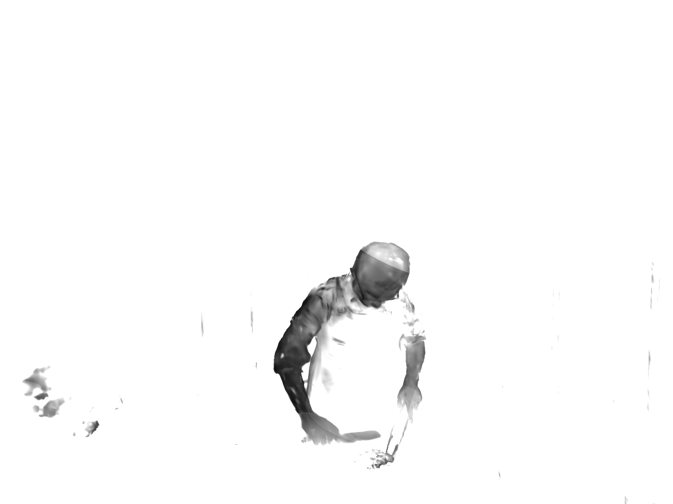
In order to more intuitively comprehend the temporal distribution of the fitted 4D Gaussian, Figure 6 presents a visualization of mean and variance in the time dimension, by which the marginal distribution on of 4D Gaussians can be completely described. It can be observed that these statistics naturally form a mask to delineate dynamic and static regions, where the background Gaussians have a large variance in the time dimension, which means they are able to cover a long time period. Actually, as shown in Figure 7, the background Gaussians are able to be active throughout the entire time span of the scene, which allows the total number of Gaussians to grow very restrained with the video length extending.
Moreover, considering that we filter the Gaussians according to the marginal probability at a negligible time cost before the frustum culling, the number of Gaussians actually participated in the rendering of each frame is nearly constant, and thus the rendering speed tends to remain stable with the increase of the video length. This locality instead makes our approach friendly to long videos in terms of rendering speed.
More ablations
To examine whether modeling the spatiotemporal evolution of Gaussian’s appearance is helpful, we ablate 4DSH in the second row of Table III. Compared to the result of our default setting, we can find there is indeed a decline in the rendering quality. Moreover, when turning our attention to 4D spacetime, we realize that over-reconstruction may occur in more than just space. Thus, we allow the Gaussian to split in time by sampling new positions using complete 4D Gaussian as PDF. The last two rows in Table III verified the effectiveness of the densification in time.
VIII-D Experiments for the compact 4D Gaussian
VIII-D1 Gaussian attributes compression
| Scaling & Rotation | Position | Opacity | Color | |||||||||
| PSNR | SSIM | Storge | PSNR | SSIM | Storge | PSNR | SSIM | Storge | PSNR | SSIM | Storge | |
| 4DGS | PSNR: 33.96 | SSIM: 0.9797 | Storge: 1183.21MB | |||||||||
| +R-VQ | -0.49 | -0.0020 | -71.88% | - | - | -0.44 | -0.0015 | -96.87% | ||||
| +8-bit quant. | - | - | -0.00 | -0.0000 | -75.00% | - | ||||||
| +16-bit quant. | - | -0.01 | -0.0001 | -50.00% | - | - | ||||||
| +fine-tune | +0.02 | +0.0003 | -71.88% | +0.10 | +0.0007 | -50.00% | +0.11 | +0.0007 | -75.00% | +0.08 | +0.0007 | -96.87% |
| +encode | +0.02 | +0.0003 | -72.56% | - | +0.11 | +0.0007 | -76.33% | +0.08 | +0.0007 | -98.93% | ||
| +All | PSNR: 33.86 (-0.1) | SSIM: 0.9795 (-0.0002) | Storge: 56.74MB (-95.20%) | |||||||||
Implementation details
The baseline model adopts the default settings except for increasing the opacity pruning threshold to 0.05. For scaling, we employ an R-VQ model with codebooks each containing entries. The codebook parameters are optimized during extra steps with a learning rate on the pre-trained baseline model. Both rotation parameters share the same R-VQ model also consisting of codebooks with 64 entries, optimized for steps at learning rate. For appearance modeling, the direct and rest components adopt codebooks with entries and codebooks with entries, respectively. For opacity, we use quantization-aware fine-tuning with -bit Min-Max Quantization [38, 103] to fine-tune for iterations with learning rate. All experiments are conducted on the Cut Roasted Beef from [4].
Results
In Table IV, we validate the effects of the parameter compression strategy introduced in Section IV-B. For the shape-related attributes, i.e., rotation and scaling, the R-VQ reduces their memory from bits to bits for Gaussians. Since the real scenes could contain millions of Gaussians, this process can achieve around compression rates with negligible damage to quality. After VQ and Huffman encoding on the codebook indices, their storage consumption decreases from 88.19 MB to 24.20 MB. Although it leads to a 0.49 dB PSNR drop, the post-finetuning of the codebook entries can recover the PSNR by 0.51 dB. Similarly, the size of color-related parameters decreases by nearly 1000 MB with little PSNR drop. Quantization of position and opacity parameters reduces storage overhead by 50% and 75% respectively, with a negligible performance cost. And the post-finetuning even yields better performance than the original model. By utilizing all of the above strategies together, the total memory overhead decreases from 1183.21 MB to 56.74 MB, while almost maintaining the same rendering quality.
VIII-D2 Culling redundant Gaussians

| Opacity threshold | Scene | PSNR | SSIM | #Points |
| 0.005 | Sear Steak | 33.53 | 0.963 | 2.54M |
| Cut Roasted Beef | 33.87 | 0.980 | 3.05M | |
| 0.05 | Sear Steak | 33.81 | 0.962 | 1.26M |
| Cut Roasted Beef | 34.02 | 0.980 | 1.49M |
For redundant primitive pruning, we compare two methods for eliminating Gaussians: the volume mask [35] and vanilla opacity with varying thresholds from conservative to aggressive. This comparison clearly demonstrates the trade-off between performance and storage cost under different criteria. Specifically, we set in equation (21) for the volume mask and use opacity thresholds of 0.005 and 0.05. The pruning experiments are conducted on the Sear Steak sequence from the Plenoptic Video dataset.
As shown in Figure 8, the total number of Gaussian points decreases rapidly after the stop of densification when using the volume mask, while the PSNR remains stable, indicating that the mask pruning technique effectively removes redundant Gaussians. This results in a reduction in the total number of points, from 1.26M to 0.51M. Table V provides the detailed quantitative results. A higher opacity threshold eliminates floaters in the scene, leading to a higher PSNR (33.46 vs. 30.48) and decreasing the number of Gaussian points from 2.62M to 1.26M. Additionally, applying mask pruning further reduces the number of redundant Gaussians while preserving similar rendering quality. Given that the mask pruning technique introduces minimal additional computational overhead, we choose to use it with a threshold of 0.05 as the default method for reducing the number of Gaussians.
VIII-D3 Structured 4D Gaussians
| Scene | w/ structured | PSNR | SSIM | #Points |
| Bouncingballs | ✗ | 33.54 | 0.982 | 127K |
| ✓ | 37.78 | 0.990 | 5.67K | |
| Lego | ✗ | 25.56 | 0.938 | 389K |
| ✓ | 30.43 | 0.958 | 15.6K |
In Table VI, we verify the effectiveness of structured 4D Gaussians in reducing the number of primitives and the performance gains in monocular dynamic scenes. Compared to full 4DGS, there is a substantial reduction in the number of final 4D primitives to be stored after optimization, thanks to the reduction of its redundancy in space and time as well as the elimination of a large number of Gaussian caused by overfitting. It also brings considerable performance improvements by better aggregating multi-frame supervision.
VIII-E Experiments on dynamic urban scenes
| Method | PSNR | SSIM | LPIPS |
| - Scene reconstruction | |||
| D2NeRF [104] | 24.35 | 0.645 | - |
| HyperNeRF [105] | 25.17 | 0.688 | - |
| EmerNeRF [61] | 28.87 | 0.814 | - |
| MARS [52] | 28.24 | 0.866 | 0.252 |
| 3DGS [24] | 28.47 | 0.876 | 0.136 |
| S3Gaussian [62] | 31.35 | 0.911 | 0.106 |
| 4DGS (Ours) | 35.04 | 0.943 | 0.057 |
| - Novel view synthesis | |||
| D2NeRF [104] | 24.17 | 0.642 | - |
| HyperNeRF [105] | 24.71 | 0.682 | - |
| EmerNeRF [61] | 27.62 | 0.792 | - |
| MARS [52] | 26.61 | 0.796 | 0.305 |
| 3DGS [24] | 25.14 | 0.813 | 0.165 |
| S3Gaussian [62] | 27.44 | 0.857 | 0.137 |
| 4DGS (Ours) | 28.67 | 0.868 | 0.102 |
 |
 |
 |
 |
VIII-E1 Experimental setup
We evaluate the Waymo-NOTR Dynamic-32 split curated by [61], with 32 sequences of calibrated images captured by five pinhole cameras and LiDAR point clouds. These driving sequences contain rich challenging dynamic objects. Following the common practice, we divide each of them into clips of 50 consecutive frames for training and use images at resolution from three frontal cameras in both training and evaluation. For reconstruction, we train and test on all frames of each clip. For novel view synthesis, we take out one frame every ten frames for testing and train on the remaining frames. The warm-up steps for all experiments is set to 3,000 unless otherwise specified.
VIII-E2 Results
Table VII shows that our 4DGS (see Section V) can achieve comparable and even better performance against those complex pipelines specifically designed for urban scenes. Meanwhile, our fully explicit and unified representation supports highly efficient rendering, achieving superior efficiency over all competitors except 3DGS. As shown in Figure 9, 4DGS works well under diverse lighting and weather conditions. It faithfully reconstructs high-frequency texture details and correctly models the geometry for both dynamic and static regions.
VIII-E3 Ablations
| Settings | Recon. | NVS | ||
| PSNR | SSIM | PSNR | SSIM | |
| 4DGS | 37.05 | 0.964 | 29.45 | 0.880 |
| (a) + | 36.98 | 0.960 | 29.59 | 0.884 |
| (b) + | 36.17 | 0.961 | 30.22 | 0.898 |
| (c) + | 36.08 | 0.956 | 30.49 | 0.904 |
| (d) +Rand. Perturb. | 35.60 | 0.953 | 30.59 | 0.907 |
| (e) +3D Warm-up | 36.08 | 0.956 | 31.46 | 0.915 |
| (f) + (Full) | 36.94 | 0.959 | 31.62 | 0.916 |
We conduct ablation studies to investigate the impact of modifications for driving scenes. From Table VIII, we can draw these observations: (a) Introducing LiDAR supervision slightly increases performance for novel view synthesis, as relying solely on multi-view images to reconstruct the accurate geometry of textureless regions such as road surfaces is inherently difficult without additional prior constraints. (b) While strong capability of 4DGS, it is challenging to constrain the behavior of Gaussians at a very novel time without static prior. effectively addresses this by encouraging sparse motion and significantly boosts the rendering quality in novel views. (c) Applying regularization to the covariance in time dimension can increase the lifetime of the 4D Gaussian, enabling it to better utilize multi-view supervision. (d) Temporal random perturbation further reduces undesired motions, effectively enhancing the performance for novel view synthesis. (e) Warm-up and (f) both slightly improve the performance of novel view synthesis by introducing reasonable priors about motion.
VIII-F Experiments for generative 4D Gaussian
| Representation | Representative methods | Total time (time per iter) | CLIP | LPIPS |
| C-DyNeRF [14] | Consistent4D [14] | 3h (11s) | 0.875 | 0.147 |
| Deform-GS [42] | DG4D [73] 4DGen [74] STAG4D [75] | 22m (2.6s) | 0.898 | 0.133 |
| 4DGS (Ours) | Efficient4D [76] | 9m30s (1.1s) | 0.905 | 0.129 |


Dataset
Consistent4D test dataset [14]: comprises seven videos with 32 frames, each containing ground truth images from four viewpoints at every timestamp. In this dataset, we initialize 50,000 random points inside a sphere of radius 0.5 with uniformly distributed timestamps.
Implementation details
Competitors
We include cascade dynamic NeRF (C-DyNeRF) introduced in [14] and Deform-GS [42] as alternative representations for comparison. Due to different convergence speeds, we train C-DyNeRF for 1000 iterations and Deform-GS for 500 iterations. The other training settings follow those specified in the respective papers.
Metrics
For each 4D representation, we report the total generation time needed for complete convergence and the time required for a single training iteration. We report the CLIP similarity and LPIPS between rendered images and groundtruth images.
Results
Table IX reports the results on the Consistent4D test dataset. Our 4DGS significantly surpasses all alternatives in terms of both generation time and quality. Figure 11 shows that 4DGS is fastest to converge. We note C-DyNeRF fails to converge in 500 iterations, whereas Gaussian-based representations succeed.
VIII-G Experiments for 4D Gaussian segmentation
We evaluate 4DGS for 4D segmentation (see Section VII) with focus on visualization.
Implementation details
We set feature dimensions and in k-nearest neighbors. We train the features and scale mapping based on compact 4DGS (see Section IV), pre-trained on the Sear Steak sequence from the Plenoptic Video dataset. The training is conducted with 10,000 iterations at a batch size of 1. In inference, as [81] we cluster Gaussians in 4D space based on the learned features using HDBSCAN, achieving automatic scene decomposition. For 4D segments, we first extract the 2D feature from the rendered feature map at a user-specific 2D point and then filter the 4D Gaussians whose smoothed scale-gated feature similarity with the query feature is below a certain threshold (typically 0.8). The filtered 4D Gaussians represent a certain component most similar to the 2D point and can be rendered from any views at any timestamp. For both scene decomposition and 4D segments, we adjust the input scale from 0 to 1 to achieve multi-granularity segmentation.
Results
Figure 10 shows the multi-granularity segmentation results. The learned features enable the 4D Gaussians to cluster automatically and adaptively as the scale varies. At scale 0, individual elements like the man’s hair, clothing, and arms are distinctly segmented. As the scale increases to 1, the entire figure of the man is segmented as a whole. This multi-granularity segmentation capability also extends to 4D segments. For example, the Gaussians representing the man’s whole body, head, or arm can be identified at different scales with minimal blurry floaters.
IX Conclusion
We introduced 4D Gaussian Splatting (4DGS), a novel framework for dynamic 3D scene representation, formulated as a spatio-temporal 4D volume learning problem. By leveraging 4D Gaussian primitives with anisotropic ellipses and 4D spherical harmonics, 4DGS effectively captures complex scene dynamics and enables real-time, high-resolution, photorealistic novel view rendering. To improve efficiency, we proposed compact variants that reduce memory usage and prevent overfitting. Extensive experiments validate the visual quality and efficiency of 4DGS across tasks like novel view synthesis, 4D generation, and scene understanding, proving its versatility across real and synthetic scenarios.
References
- [1] B. Mildenhall, P. P. Srinivasan, M. Tancik, J. T. Barron, R. Ramamoorthi, and R. Ng, “Nerf: Representing scenes as neural radiance fields for view synthesis,” in European Conference on Computer Vision, 2020.
- [2] J. T. Barron, B. Mildenhall, M. Tancik, P. Hedman, R. Martin-Brualla, and P. P. Srinivasan, “Mip-nerf: A multiscale representation for anti-aliasing neural radiance fields,” in IEEE International Conference on Computer Vision, 2021.
- [3] D. Verbin, P. Hedman, B. Mildenhall, T. Zickler, J. T. Barron, and P. P. Srinivasan, “Ref-nerf: Structured view-dependent appearance for neural radiance fields,” in IEEE Conference on Computer Vision and Pattern Recognition, 2022.
- [4] T. Li, M. Slavcheva, M. Zollhoefer, S. Green, C. Lassner, C. Kim, T. Schmidt, S. Lovegrove, M. Goesele, R. Newcombe et al., “Neural 3d video synthesis from multi-view video,” in IEEE Conference on Computer Vision and Pattern Recognition, 2022.
- [5] F. Wang, S. Tan, X. Li, Z. Tian, and H. Liu, “Mixed neural voxels for fast multi-view video synthesis,” in IEEE International Conference on Computer Vision, 2023.
- [6] S. Fridovich-Keil, G. Meanti, F. R. Warburg, B. Recht, and A. Kanazawa, “K-planes: Explicit radiance fields in space, time, and appearance,” in IEEE Conference on Computer Vision and Pattern Recognition, 2023.
- [7] A. Cao and J. Johnson, “Hexplane: A fast representation for dynamic scenes,” in IEEE Conference on Computer Vision and Pattern Recognition, 2023.
- [8] B. Attal, J.-B. Huang, C. Richardt, M. Zollhoefer, J. Kopf, M. O’Toole, and C. Kim, “HyperReel: High-fidelity 6-DoF video with ray-conditioned sampling,” in IEEE Conference on Computer Vision and Pattern Recognition, 2023.
- [9] A. Pumarola, E. Corona, G. Pons-Moll, and F. Moreno-Noguer, “D-nerf: Neural radiance fields for dynamic scenes,” in IEEE Conference on Computer Vision and Pattern Recognition, 2021.
- [10] L. Song, A. Chen, Z. Li, Z. Chen, L. Chen, J. Yuan, Y. Xu, and A. Geiger, “Nerfplayer: A streamable dynamic scene representation with decomposed neural radiance fields,” IEEE Transactions on Visualization and Computer Graphics, 2023.
- [11] J. Abou-Chakra, F. Dayoub, and N. Sünderhauf, “Particlenerf: Particle based encoding for online neural radiance fields in dynamic scenes,” arXiv preprint, 2022.
- [12] J. Luiten, G. Kopanas, B. Leibe, and D. Ramanan, “Dynamic 3d gaussians: Tracking by persistent dynamic view synthesis,” in 3DV, 2024.
- [13] Z. Yang, H. Yang, Z. Pan, X. Zhu, and L. Zhang, “Real-time photorealistic dynamic scene representation and rendering with 4d gaussian splatting,” in International Conference on Learning Representations, 2024.
- [14] Y. Jiang, L. Zhang, J. Gao, W. Hu, and Y. Yao, “Consistent4d: Consistent 360° dynamic object generation from monocular video,” in International Conference on Learning Representations, 2024.
- [15] A. Chen, Z. Xu, A. Geiger, J. Yu, and H. Su, “Tensorf: Tensorial radiance fields,” in European Conference on Computer Vision, 2022.
- [16] C. Sun, M. Sun, and H.-T. Chen, “Direct voxel grid optimization: Super-fast convergence for radiance fields reconstruction,” in IEEE Conference on Computer Vision and Pattern Recognition, 2022.
- [17] T. Hu, S. Liu, Y. Chen, T. Shen, and J. Jia, “Efficientnerf efficient neural radiance fields,” in IEEE Conference on Computer Vision and Pattern Recognition, 2022.
- [18] A. Chen, Z. Xu, X. Wei, S. Tang, H. Su, and A. Geiger, “Factor fields: A unified framework for neural fields and beyond,” arXiv preprint, 2023.
- [19] S. Fridovich-Keil, A. Yu, M. Tancik, Q. Chen, B. Recht, and A. Kanazawa, “Plenoxels: Radiance fields without neural networks,” in IEEE Conference on Computer Vision and Pattern Recognition, 2022.
- [20] T. Müller, A. Evans, C. Schied, and A. Keller, “Instant neural graphics primitives with a multiresolution hash encoding,” ACM Transactions on Graphics, 2022.
- [21] K. Zhang, G. Riegler, N. Snavely, and V. Koltun, “Nerf++: Analyzing and improving neural radiance fields,” arXiv preprint, 2020.
- [22] J. T. Barron, B. Mildenhall, D. Verbin, P. P. Srinivasan, and P. Hedman, “Mip-nerf 360: Unbounded anti-aliased neural radiance fields,” in IEEE Conference on Computer Vision and Pattern Recognition, 2022.
- [23] J. T. Barron, B. Mildenhall, D. Verbin, P. P. Srinivasan, and P. Hedman, “Zip-nerf: Anti-aliased grid-based neural radiance fields,” in IEEE International Conference on Computer Vision, 2023.
- [24] B. Kerbl, G. Kopanas, T. Leimkühler, and G. Drettakis, “3d gaussian splatting for real-time radiance field rendering,” ACM Transactions on Graphics, 2023.
- [25] G. Chen and W. Wang, “A survey on 3d gaussian splatting,” arXiv preprint, 2024.
- [26] T. Wu, Y.-J. Yuan, L.-X. Zhang, J. Yang, Y.-P. Cao, L.-Q. Yan, and L. Gao, “Recent advances in 3d gaussian splatting,” Computational Visual Media, 2024.
- [27] Z. Yu, A. Chen, B. Huang, T. Sattler, and A. Geiger, “Mip-splatting: Alias-free 3d gaussian splatting,” in IEEE Conference on Computer Vision and Pattern Recognition, 2024.
- [28] Z. Liang, Q. Zhang, W. Hu, Y. Feng, L. Zhu, and K. Jia, “Analytic-splatting: Anti-aliased 3d gaussian splatting via analytic integration,” arXiv preprint, 2024.
- [29] K. Cheng, X. Long, K. Yang, Y. Yao, W. Yin, Y. Ma, W. Wang, and X. Chen, “Gaussianpro: 3d gaussian splatting with progressive propagation,” in International Conference on Machine Learning, 2024.
- [30] X. Song, J. Zheng, S. Yuan, H.-a. Gao, J. Zhao, X. He, W. Gu, and H. Zhao, “Sa-gs: Scale-adaptive gaussian splatting for training-free anti-aliasing,” arXiv preprint arXiv:2403.19615, 2024.
- [31] Z. Ye, W. Li, S. Liu, P. Qiao, and Y. Dou, “Absgs: Recovering fine details in 3d gaussian splatting,” in ACM Multimedia Conference, 2024.
- [32] A. Guédon and V. Lepetit, “Sugar: Surface-aligned gaussian splatting for efficient 3d mesh reconstruction and high-quality mesh rendering,” in IEEE Conference on Computer Vision and Pattern Recognition, 2024.
- [33] B. Huang, Z. Yu, A. Chen, A. Geiger, and S. Gao, “2d gaussian splatting for geometrically accurate radiance fields,” in ACM SIGGRAPH 2024 Conference Papers, 2024, pp. 1–11.
- [34] Z. Yu, T. Sattler, and A. Geiger, “Gaussian opacity fields: Efficient and compact surface reconstruction in unbounded scenes,” arXiv preprint, 2024.
- [35] J. C. Lee, D. Rho, X. Sun, J. H. Ko, and E. Park, “Compact 3d gaussian representation for radiance field,” in IEEE Conference on Computer Vision and Pattern Recognition, 2024.
- [36] N. Zeghidour, A. Luebs, A. Omran, J. Skoglund, and M. Tagliasacchi, “Soundstream: An end-to-end neural audio codec,” in IEEE/ACM Transactions on Audio, Speech, and Language Processing, 2021.
- [37] P. Papantonakis, G. Kopanas, B. Kerbl, A. Lanvin, and G. Drettakis, “Reducing the memory footprint of 3d gaussian splatting,” in Proceedings of the ACM on Computer Graphics and Interactive Techniques, 2024.
- [38] S. Niedermayr, J. Stumpfegger, and R. Westermann, “Compressed 3d gaussian splatting for accelerated novel view synthesis,” in IEEE Conference on Computer Vision and Pattern Recognition, 2024.
- [39] T. Lu, M. Yu, L. Xu, Y. Xiangli, L. Wang, D. Lin, and B. Dai, “Scaffold-gs: Structured 3d gaussians for view-adaptive rendering,” in IEEE Conference on Computer Vision and Pattern Recognition, 2024.
- [40] Y. Chen, Q. Wu, J. Cai, M. Harandi, and W. Lin, “Hac: Hash-grid assisted context for 3d gaussian splatting compression,” in European Conference on Computer Vision, 2024.
- [41] Z. Yang, X. Gao, W. Zhou, S. Jiao, Y. Zhang, and X. Jin, “Deformable 3d gaussians for high-fidelity monocular dynamic scene reconstruction,” in IEEE Conference on Computer Vision and Pattern Recognition, 2023.
- [42] G. Wu, T. Yi, J. Fang, L. Xie, X. Zhang, W. Wei, W. Liu, Q. Tian, and W. Xinggang, “4d gaussian splatting for real-time dynamic scene rendering,” in IEEE Conference on Computer Vision and Pattern Recognition, 2024.
- [43] Y. Liang, N. Khan, Z. Li, T. Nguyen-Phuoc, D. Lanman, J. Tompkin, and L. Xiao, “Gaufre: Gaussian deformation fields for real-time dynamic novel view synthesis,” arXiv preprint, 2023.
- [44] A. Kratimenos, J. Lei, and K. Daniilidis, “Dynmf: Neural motion factorization for real-time dynamic view synthesis with 3d gaussian splatting,” arXiv preprint, 2023.
- [45] Y. Duan, F. Wei, Q. Dai, Y. He, W. Chen, and B. Chen, “4d-rotor gaussian splatting: Towards efficient novel view synthesis for dynamic scenes,” in ACM SIGGRAPH 2024 Conference Papers, 2024.
- [46] Y.-H. Huang, Y.-T. Sun, Z. Yang, X. Lyu, Y.-P. Cao, and X. Qi, “Sc-gs: Sparse-controlled gaussian splatting for editable dynamic scenes,” in IEEE Conference on Computer Vision and Pattern Recognition, 2024.
- [47] Z. Xu, Y. Xu, Z. Yu, S. Peng, J. Sun, H. Bao, and X. Zhou, “Representing long volumetric video with temporal gaussian hierarchy,” in ACM Transactions on Graphics, 2024.
- [48] A. Dosovitskiy, G. Ros, F. Codevilla, A. Lopez, and V. Koltun, “Carla: An open urban driving simulator,” in Conference on Robot Learning, 2017.
- [49] S. Shah, D. Dey, C. Lovett, and A. Kapoor, “Airsim: High-fidelity visual and physical simulation for autonomous vehicles,” in Field and Service Robotics: Results of the 11th International Conference, 2018.
- [50] Y. Chen, F. Rong, S. Duggal, S. Wang, X. Yan, S. Manivasagam, S. Xue, E. Yumer, and R. Urtasun, “Geosim: Realistic video simulation via geometry-aware composition for self-driving,” in IEEE Conference on Computer Vision and Pattern Recognition, 2021.
- [51] Z. Xie, J. Zhang, W. Li, F. Zhang, and L. Zhang, “S-nerf: Neural radiance fields for street views,” in International Conference on Learning Representations, 2023.
- [52] Z. Wu, T. Liu, L. Luo, Z. Zhong, J. Chen, H. Xiao, C. Hou, H. Lou, Y. Chen, R. Yang et al., “Mars: An instance-aware, modular and realistic simulator for autonomous driving,” in CAAI International Conference on Artificial Intelligence. Springer, 2023.
- [53] Z. Yang, Y. Chen, J. Wang, S. Manivasagam, W.-C. Ma, A. J. Yang, and R. Urtasun, “Unisim: A neural closed-loop sensor simulator,” in IEEE Conference on Computer Vision and Pattern Recognition, 2023.
- [54] J. Guo, N. Deng, X. Li, Y. Bai, B. Shi, C. Wang, C. Ding, D. Wang, and Y. Li, “Streetsurf: Extending multi-view implicit surface reconstruction to street views,” arXiv preprint, 2023.
- [55] Y. Chen, J. Zhang, Z. Xie, W. Li, F. Zhang, J. Lu, and L. Zhang, “S-nerf++: Autonomous driving simulation via neural reconstruction and generation,” arXiv preprint, 2024.
- [56] J. Lin, Z. Li, X. Tang, J. Liu, S. Liu, J. Liu, Y. Lu, X. Wu, S. Xu, Y. Yan et al., “Vastgaussian: Vast 3d gaussians for large scene reconstruction,” in IEEE Conference on Computer Vision and Pattern Recognition, 2024.
- [57] Y. Yan, H. Lin, C. Zhou, W. Wang, H. Sun, K. Zhan, X. Lang, X. Zhou, and S. Peng, “Street gaussians for modeling dynamic urban scenes,” in European Conference on Computer Vision, 2024.
- [58] Y. Liu, H. Guan, C. Luo, L. Fan, J. Peng, and Z. Zhang, “Citygaussian: Real-time high-quality large-scale scene rendering with gaussians,” arXiv preprint, 2024.
- [59] H. Zhou, J. Shao, L. Xu, D. Bai, W. Qiu, B. Liu, Y. Wang, A. Geiger, and Y. Liao, “Hugs: Holistic urban 3d scene understanding via gaussian splatting,” in IEEE Conference on Computer Vision and Pattern Recognition, 2024.
- [60] H. Turki, J. Y. Zhang, F. Ferroni, and D. Ramanan, “Suds: Scalable urban dynamic scenes,” in IEEE Conference on Computer Vision and Pattern Recognition, 2023.
- [61] J. Yang, B. Ivanovic, O. Litany, X. Weng, S. W. Kim, B. Li, T. Che, D. Xu, S. Fidler, M. Pavone et al., “Emernerf: Emergent spatial-temporal scene decomposition via self-supervision,” in International Conference on Learning Representations, 2023.
- [62] N. Huang, X. Wei, W. Zheng, P. An, M. Lu, W. Zhan, M. Tomizuka, K. Keutzer, and S. Zhang, “S^ 3gaussian: Self-supervised street gaussians for autonomous driving,” arXiv preprint, 2024.
- [63] Y. Chen, C. Gu, J. Jiang, X. Zhu, and L. Zhang, “Periodic vibration gaussian: Dynamic urban scene reconstruction and real-time rendering,” arXiv preprint, 2023.
- [64] A. Jain, B. Mildenhall, J. T. Barron, P. Abbeel, and B. Poole, “Zero-shot text-guided object generation with dream fields,” in IEEE Conference on Computer Vision and Pattern Recognition, 2022.
- [65] B. Poole, A. Jain, J. T. Barron, and B. Mildenhall, “Dreamfusion: Text-to-3d using 2d diffusion,” in IEEE Conference on Computer Vision and Pattern Recognition, 2023.
- [66] C.-H. Lin, J. Gao, L. Tang, T. Takikawa, X. Zeng, X. Huang, K. Kreis, S. Fidler, M.-Y. Liu, and T.-Y. Lin, “Magic3d: High-resolution text-to-3d content creation,” in IEEE Conference on Computer Vision and Pattern Recognition, 2023.
- [67] J. Tang, J. Ren, H. Zhou, Z. Liu, and G. Zeng, “Dreamgaussian: Generative gaussian splatting for efficient 3d content creation,” in International Conference on Learning Representations, 2024.
- [68] T. Yi, J. Fang, J. Wang, G. Wu, L. Xie, X. Zhang, W. Liu, Q. Tian, and X. Wang, “Gaussiandreamer: Fast generation from text to 3d gaussians by bridging 2d and 3d diffusion models,” in IEEE Conference on Computer Vision and Pattern Recognition, 2024.
- [69] Z. Chen, F. Wang, Y. Wang, and H. Liu, “Text-to-3d using gaussian splatting,” in IEEE Conference on Computer Vision and Pattern Recognition, 2024.
- [70] C. Gu, Z. Yang, Z. Pan, X. Zhu, and L. Zhang, “Tetrahedron splatting for 3d generation,” arXiv preprint, 2024.
- [71] S. Bahmani, I. Skorokhodov, V. Rong, G. Wetzstein, L. Guibas, P. Wonka, S. Tulyakov, J. J. Park, A. Tagliasacchi, and D. B. Lindell, “4d-fy: Text-to-4d generation using hybrid score distillation sampling,” in IEEE Conference on Computer Vision and Pattern Recognition, 2024.
- [72] U. Singer, S. Sheynin, A. Polyak, O. Ashual, I. Makarov, F. Kokkinos, N. Goyal, A. Vedaldi, D. Parikh, J. Johnson et al., “Text-to-4d dynamic scene generation,” in International Conference on Machine Learning, 2023.
- [73] J. Ren, L. Pan, J. Tang, C. Zhang, A. Cao, G. Zeng, and Z. Liu, “Dreamgaussian4d: Generative 4d gaussian splatting,” arXiv preprint, 2023.
- [74] Y. Yin, D. Xu, Z. Wang, Y. Zhao, and Y. Wei, “4dgen: Grounded 4d content generation with spatial-temporal consistency,” arXiv preprint, 2023.
- [75] Y. Zeng, Y. Jiang, S. Zhu, Y. Lu, Y. Lin, H. Zhu, W. Hu, X. Cao, and Y. Yao, “Stag4d: Spatial-temporal anchored generative 4d gaussians,” in European Conference on Computer Vision, 2024.
- [76] Z. Pan, Z. Yang, X. Zhu, and L. Zhang, “Efficient4d: Fast dynamic 3d object generation from a single-view video,” arXiv preprint, 2024.
- [77] Z. Wu, C. Yu, Y. Jiang, C. Cao, F. Wang, and X. Bai, “Sc4d: Sparse-controlled video-to-4d generation and motion transfer,” in European Conference on Computer Vision, 2024.
- [78] Q. Gao, Q. Xu, Z. Cao, B. Mildenhall, W. Ma, L. Chen, D. Tang, and U. Neumann, “Gaussianflow: Splatting gaussian dynamics for 4d content creation,” arXiv preprint, 2024.
- [79] A. Kirillov, E. Mintun, N. Ravi, H. Mao, C. Rolland, L. Gustafson, T. Xiao, S. Whitehead, A. C. Berg, W.-Y. Lo, P. Dollar, and R. Girshick, “Segment anything,” in IEEE International Conference on Computer Vision, 2023.
- [80] S. Ji, G. Wu, J. Fang, J. Cen, T. Yi, W. Liu, Q. Tian, and X. Wang, “Segment any 4d gaussians,” arXiv preprint, 2024.
- [81] J. Cen, J. Fang, C. Yang, L. Xie, X. Zhang, W. Shen, and Q. Tian, “Segment any 3d gaussians,” arXiv preprint, 2023.
- [82] S. Zhi, T. Laidlow, S. Leutenegger, and A. J. Davison, “In-place scene labelling and understanding with implicit scene representation,” in IEEE International Conference on Computer Vision, 2021.
- [83] C. M. Kim, M. Wu, J. Kerr, K. Goldberg, M. Tancik, and A. Kanazawa, “Garfield: Group anything with radiance fields,” in IEEE Conference on Computer Vision and Pattern Recognition, 2024.
- [84] J. Cen, Z. Zhou, J. Fang, W. Shen, L. Xie, D. Jiang, X. Zhang, Q. Tian et al., “Segment anything in 3d with nerfs,” in Advances in Neural Information Processing Systems, 2023.
- [85] M. Ye, M. Danelljan, F. Yu, and L. Ke, “Gaussian grouping: Segment and edit anything in 3d scenes,” arXiv preprint, 2023.
- [86] H. Ying, Y. Yin, J. Zhang, F. Wang, T. Yu, R. Huang, and L. Fang, “Omniseg3d: Omniversal 3d segmentation via hierarchical contrastive learning,” in IEEE Conference on Computer Vision and Pattern Recognition, 2024.
- [87] Y. Chen, Z. Chen, C. Zhang, F. Wang, X. Yang, Y. Wang, Z. Cai, L. Yang, H. Liu, and G. Lin, “Gaussianeditor: Swift and controllable 3d editing with gaussian splatting,” in IEEE Conference on Computer Vision and Pattern Recognition, 2024.
- [88] M. Zwicker, H. Pfister, J. Van Baar, and M. Gross, “Ewa splatting,” IEEE Transactions on Visualization and Computer Graphics, 2002.
- [89] D. A. Huffman, “A method for the construction of minimum-redundancy codes,” Proceedings of the IRE, 1952.
- [90] E. Xie, W. Wang, Z. Yu, A. Anandkumar, J. M. Alvarez, and P. Luo, “Segformer: Simple and efficient design for semantic segmentation with transformers,” in Advances in Neural Information Processing Systems, 2021.
- [91] Y. Liu, C. Lin, Z. Zeng, X. Long, L. Liu, T. Komura, and W. Wang, “Syncdreamer: Generating multiview-consistent images from a single-view image,” in International Conference on Learning Representations, 2024.
- [92] R. Liu, R. Wu, B. Van Hoorick, P. Tokmakov, S. Zakharov, and C. Vondrick, “Zero-1-to-3: Zero-shot one image to 3d object,” in IEEE International Conference on Computer Vision, 2023.
- [93] S. AI, “Stable zero123: Quality 3d object generation from single images,” https://stability.ai/news/stable-zero123-3d-generation, 2023.
- [94] R. Zhang, P. Isola, A. A. Efros, E. Shechtman, and O. Wang, “The unreasonable effectiveness of deep features as a perceptual metric,” in IEEE Conference on Computer Vision and Pattern Recognition, 2018.
- [95] A. Krizhevsky, I. Sutskever, and G. E. Hinton, “Imagenet classification with deep convolutional neural networks,” in Advances in Neural Information Processing Systems, 2012.
- [96] K. Simonyan and A. Zisserman, “Very deep convolutional networks for large-scale image recognition,” arXiv preprint, 2014.
- [97] S. Lombardi, T. Simon, J. Saragih, G. Schwartz, A. Lehrmann, and Y. Sheikh, “Neural volumes: learning dynamic renderable volumes from images,” ACM Transactions on Graphics, 2019.
- [98] B. Mildenhall, P. P. Srinivasan, R. Ortiz-Cayon, N. K. Kalantari, R. Ramamoorthi, R. Ng, and A. Kar, “Local light field fusion: Practical view synthesis with prescriptive sampling guidelines,” ACM Transactions on Graphics, 2019.
- [99] L. Li, Z. Shen, Z. Wang, L. Shen, and P. Tan, “Streaming radiance fields for 3d video synthesis,” in Advances in Neural Information Processing Systems, 2022.
- [100] J. Fang, T. Yi, X. Wang, L. Xie, X. Zhang, W. Liu, M. Nießner, and Q. Tian, “Fast dynamic radiance fields with time-aware neural voxels,” in SIGGRAPH Asia Conference Papers, 2022.
- [101] W. Gan, H. Xu, Y. Huang, S. Chen, and N. Yokoya, “V4d: Voxel for 4d novel view synthesis,” IEEE Transactions on Visualization and Computer Graphics, 2024.
- [102] X. Shi, Z. Huang, W. Bian, D. Li, M. Zhang, K. C. Cheung, S. See, H. Qin, J. Dai, and H. Li, “Videoflow: Exploiting temporal cues for multi-frame optical flow estimation,” arXiv preprint, 2023.
- [103] M. Rastegari, V. Ordonez, J. Redmon, and A. Farhadi, “Xnor-net: Imagenet classification using binary convolutional neural networks,” in European Conference on Computer Vision, 2016.
- [104] T. Wu, F. Zhong, A. Tagliasacchi, F. Cole, and C. Oztireli, “D^ 2nerf: Self-supervised decoupling of dynamic and static objects from a monocular video,” in Advances in Neural Information Processing Systems, 2022.
- [105] K. Park, U. Sinha, P. Hedman, J. T. Barron, S. Bouaziz, D. B. Goldman, R. Martin-Brualla, and S. M. Seitz, “Hypernerf: A higher-dimensional representation for topologically varying neural radiance fields,” in ACM Transactions on Graphics, 2021.