3D Scene Flow Estimation on Pseudo-LiDAR: Bridging the Gap on Estimating Point Motion
Abstract
3D scene flow characterizes how the points at the current time flow to the next time in the 3D Euclidean space, which possesses the capacity to infer autonomously the non-rigid motion of all objects in the scene. The previous methods for estimating scene flow from images have limitations, which split the holistic nature of 3D scene flow by estimating optical flow and disparity separately. Learning 3D scene flow from point clouds also faces the difficulties of the gap between synthesized and real data and the sparsity of LiDAR point clouds. In this paper, the generated dense depth map is utilized to obtain explicit 3D coordinates, which achieves direct learning of 3D scene flow from 2D images. The stability of the predicted scene flow is improved by introducing the dense nature of 2D pixels into the 3D space. Outliers in the generated 3D point cloud are removed by statistical methods to weaken the impact of noisy points on the 3D scene flow estimation task. Disparity consistency loss is proposed to achieve more effective unsupervised learning of 3D scene flow. The proposed method of self-supervised learning of 3D scene flow on real-world images is compared with a variety of methods for learning on the synthesized dataset and learning on LiDAR point clouds. The comparisons of multiple scene flow metrics are shown to demonstrate the effectiveness and superiority of introducing pseudo-LiDAR point cloud to scene flow estimation.
Index Terms:
Deep learning, 3D scene flow, pseudo-LiDAR point cloud.I Introduction
The scene flow [1] estimates the motion of 3D point in the scene, which is different from LiDAR odometry [2] that estimates the consistent pose transformation of the entire scene. 3D scene flow is more flexible. The flexibility of scene flow makes it capable of assisting in many different tasks, such as object tracking [3] and LiDAR odometry[2].
Generally, depth and optical flow together represent the scene flow in the scene flow estimation method based on 2D image [4, 5] or RGBD image[6]. Mono-SF [4] infers the scene flow of visible points using constraints on motion invariance of multi-view geometric and depth distribution of a single view. To obtain more reliable scene flow, Hur et al. [5] propagate temporal constraints to continuous multi-frame images. RAFT-3D [6] estimates the scene flow by soft grouping pixels into rigid objects. The nature of the scene flow being the 3D motion vectors is split by the methods for estimating scene flow by optical flow and pixel depth in image space. Because of the lack of explicit 3D geometry information in the image space, these methods often cause large pixel matching errors during scene flow inference. For example, two unrelated points that are far apart in 3D space may be very close to each other in the image plane. Dewan et al. [7] predict 3D scene flow from adjacent frames of LiDAR data in a without-learning method. This method requires various strong assumptions, such as that the local structure will not be deformed by the motion in the 3D scene. Some recent works [8, 9, 10, 11] learn 3D scene flow from point cloud pairs based on deep neural network. However, these methods of 3D scene flow estimation are invariably self-supervised/supervised on the synthesized dataset FlyingThings3D [12] and evaluated the generalization of the model on the real-world dataset KITTI Scene Flow [13]. The models trained on the synthesized dataset will cause accuracy degradation in the real world [9].
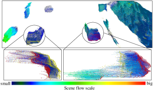
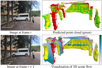
3D scene flow annotations are very scarce in real-world datasets. Some works [11, 9] proposes some excellent self-supervised losses, but these are difficult to achieve success on LiDAR signals. LiDAR signals are recognized to have two weaknesses, sparsity and point cloud distortion. Firstly, the existing self-supervised losses [9, 11] imply a strong assumption of point-by-point correspondence. But point clouds from different moments are inherently discrete. The point-by-point correspondence and the discrete nature of the point cloud are contradictory. The sparsity of the LiDAR signal further exacerbates this fact. Secondly, the data collection process for mechanical LiDAR is accompanied by motion, which results in point cloud points in the same frame not being collected at the same moment, i.e., point cloud distortion. However, 3D scene flow estimation is the process of local 3D matching, which requires accurate temporal information. Unlike the LiDAR signal, the pseudo-LiDAR signal comes from the back-projection of the dense depth map into a 3D point cloud. Almost no distortion is caused by pseudo-LiDAR due to the instantaneous capture of the image. A novel structure is designed in this paper to enable self-supervised learning of scene flow to benefit from pseudo-LiDAR. Although the spatial position of the points in the point cloud generated from the depth map is not always accurate, our method is still able to find the correspondence between the points in adjacent frames well. As shown in Fig. 1, the point clouds of adjacent frames have similar representations of same objects in the scene because the performance of the depth estimation network is unchanged. Thus the spatial features of a point at frame can easily find similar spatial features at frame and this match is usually accurate.
On the other hand, the camera is cheaper than LiDAR. Although the cost of LiDAR is shrinking year by year, there is still an undeniable cost difference between LiDAR and camera. Recently, Ouster released an inexpensive OS1-128 LiDAR, but the price still costs $18,000 [14]. The stereo camera system may provide a low-cost backup system for the LiDAR-based scheme of scene flow estimation.
In summary, our key contributions are as follows:
-
•
A self-supervised method for learning 3D scene flow from stereo images is proposed. Pseudo-LiDAR based on stereo images is introduced into 3D scene flow estimation. The method in this paper bridges the gap between 2D data and the task of estimating 3D point motion.
-
•
The sparse and distortion characteristics of the LiDAR point cloud bring errors for the calculation of existing self-supervised loss of the 3D scene flow. The introduction of the pseudo-LiDAR point cloud in this paper improves the effectiveness of these self-supervised losses because of the dense and non-distortion characteristics of the pseudo-LiDAR point cloud, which is demonstrated by experiments in this paper.
-
•
3D points with large errors caused by depth estimation are filtered out as much as possible to reduce the impact of noise points on the scene flow estimation. A novel disparity consistency loss is proposed by exploiting the coupling relationship between 3D scene flow and stereo depth estimation.
II Related Work
II-A Pseudo-LiDAR
In recent year, many works [15, 16, 17] build pseudo-LiDAR based 3D object detection pipeline. Pseudo-LiDAR has shown significant advantages in the field of object detection. Wang et al. [15] introduce pseudo-LiDAR into an existing LiDAR object detection model and demonstrate that the main reason for the performance gap between stereo and LiDAR is the representation of the data rather than the quality of the depth estimate. Pseudo-LiDAR++ [16] optimizes the structure and loss function of the depth estimation network based on Wang et al. [15] to enable the pseudo-LiDAR framework to accurately estimate distant objects. Qian et al. [17] build on Pseudo-LiDAR++ [16] to address the problem that the depth estimation network and the object detection network must be trained separately. The previous pseudo-LiDAR framework focuses more on scene perception with the single frame, while this paper focuses on the motion relationship between two frames.
II-B Scene Flow Estimation
Some works study the estimation of dense scene flow from images of consecutive frames. Mono-SF [4] proposes ProbDepthNet to estimate the pixel depth distribution of the single image. Geometric information from multiple views and depth distribution information from a single view are used to jointly estimate the scene flow. Hur et al. [5] introduce a multi-frame temporal constraint to the scene flow estimation network. Chen et al. [1] develop a coarse-grained software framework for scene-flow methods and realize real-time cross-platform embedded scene flow algorithms. In addition, Rishav et al. [18] fuse LiDAR and images to estimate dense scene flow. But they still perform feature fusion in image space. These methods rely on 2D representations and cannot learn geometric motion from explicit 3D coordinates. The pseudo-LiDAR is the bridge between the 2D signal and the 3D signal, which provides the basis for directly learning the 3D scene flow from the 2D data.
The original geometric information is preserved in the 3D point cloud, which is the preferred representation for many scene understanding applications in self-driving and robotics. Some researchers [7] estimate 3D scene flow from LiDAR point clouds by using the classical method. Dewan et al. [7] introduce local geometric constancy during the motion and introduce a triangular grid to determine the relationship of the points. Benefiting from the point cloud deep learning, some recent works [8, 9, 10, 11] propose to learn 3D scene flow from raw point clouds. FlowNet3D [8] firstly proposes the flow embedding layer which finds point correspondence and implicitly represents the 3D scene flow. FLOT [10] studies lightweight structures for optimizing scene flow estimation using optimal transport modules. PointPWC-Net [9] proposes novel learnable cost volume layers to learn 3D scene flow in a coarse-to-fine approach, and introduces three self-supervised losses to learn the 3D scene flow without accessing the ground truth. Mittal et al. [11] propose two new self-supervised loss.
III Self-Supervised Learning of the 3D Scene Flow from Pseudo-LiDAR
III-A Overview
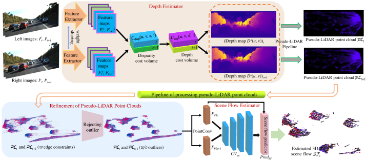
The main purpose of this paper is to recover 3D scene flow from stereo images. The stereo images are represented by and respectively. As Fig. 2, given a pair of stereo images, which contains reference frames and target frames . Each image is represented by a matrix of dimension . Depth map at time is predicted by feeding the stereo image into the depth estimation network . Each pixel value of represents the distance between a certain point in the scene and the left camera. Pseudo-LiDAR point cloud comes from back-projecting the generated depth map to a 3D point cloud, as follow:
| (1) |
where and are the horizontal and vertical focal lengths of the camera, and and are the coordinate center of the image, respectively. The 3D point coordinate in the pseudo-LiDAR point cloud is calculated by pixel coordinates , and camera intrinsics. with points and with points are generated from the depth maps and , where and are the 3D coordinates of the points. and are randomly sampled to points, respectively. The sampled pseudo-LiDAR point clouds are passed into the scene flow estimator to extract the scene flow vector for each 3D point in frame .
| (2) |
where and are the parameters of the network. represents the back-projection by Eq. (1).
It is difficult to obtain the ground truth scene flow of pseudo-LiDAR point clouds. Mining a priori knowledge from the scene itself to self-supervised learning of 3D scene flow is essential. Ideally, and estimated point cloud have the same structure. With this priori knowledge, point cloud is warped to point cloud through the predicted scene flow ,
| (3) |
Based on the consistency of and , the loss functions Eq. (7) and Eq. (10) are utilized to implement self-supervised learning. We provide the pseudocode in Algorithm 1 for our method, where , , and are described in detail in Section III-D.
III-B Depth Estimation
The disparity is the horizontal offset of the corresponding pixel in the stereo image, which represents the difference caused by viewing the same object from a stereo camera. and represent the observation of the same 3D point in space. Two cameras are connected by a line called the baseline. The distance between the object and the observation point can be calculated by knowing the disparity , the baseline length , and the horizontal focal length .
| (4) |
Disparity estimation networks such as PSMNet [19] extract deep feature maps and from and , respectively. As shown in Fig. 2, the features of and are concatenated to construct 4D tensor , namely the disparity cost volume. Then 3D tensor is calculated by feeding into the 3D convolutional neural network (CNN). The predicted pixel disparity is calculated by softmax weighting [19]. Based on the fact that disparity and depth are inversely proportional to each other, the convolution operation in the disparity cost volume has disadvantages. The same convolution kernel is applied to a few pixels with small disparity (i.e., large depth) resulting in an easy skipping and ignoring many 3D points. It is more reasonable to run the convolution kernel on the depth grid that produces the same effect on neighbor depths, rather than overemphasizing objects with large disparity (i.e., small depth) on the disparity cost volume. Based on this insight, the disparity cost volume is reconstructed as depth cost volume [16]. Finally, the depth of the pixel is calculated through a similar weighting operation as mentioned above.
The sparse LiDAR points are projected onto the 2D image as the ground truth depth map . The depth loss is constructed by minimizing the depth error:
| (5) |
represents the predicted depth map. represents smooth L1 loss.
III-C Refinement of Pseudo-LiDAR Point Clouds
Scene flow estimator cannot directly benefit from the generated original pseudo-LiDAR point clouds due to its containing many points with estimation error. Reducing the impact of these noise points on the 3D scene flow estimation is the problem to be solved.
III-C1 LiDAR and Pseudo-LiDAR for 3D Scene Flow Estimation
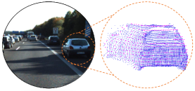
LiDAR point clouds in KITTI raw dataset [20] are captured using low-frequency (10 ) mechanical LiDAR scans. Each frame of the point cloud is collected via the rotating optical component of the LiDAR at low frequencies. This process is accompanied by the motion of the LiDAR itself and the motion of other dynamic objects. Therefore, the raw LiDAR point cloud contains a lot of distortion points. The point cloud distortion generated by its self-motion can be largely eliminated by collaborating with other sensors (e.g. inertial measurement unit). However, point cloud distortion that is caused by other dynamic objects is difficult to be eliminated, which is one of the challenges of learning 3D scene flow from LiDAR point clouds. In comparison, the sensor captures images with almost no motion distortion, which is an important advantage for recovering 3D scene flow from pseudo-LiDAR signals.
As shown in Fig. 3, the point cloud from LiDAR (64-beam) in KITTI dataset [20] is sparsely distributed on 64 horizontal beams. In contrast, pseudo-LiDAR point clouds come from dense pixel and depth values, which are inherently dense. The image size in KITTI is 1241 376. This means that the image contains 466,616 pixel points. The self-supervised learning of 3D scene flow mentioned in subsection III-A assumes that the warped point cloud and the point cloud correspond point by point. However, the disadvantage of this assumption is magnified by the sparse and discrete nature of the LiDAR point cloud. For example, Chamfer loss [9] forces the point cloud of these two frames to correspond point by point, which makes self-supervised loss over-punish the network so that it does not converge to the global optimum.
III-C2 Constraints on Pseudo-LiDAR Point Cloud Edges
A large number of incorrectly estimated points are distributed at the scene boundaries. For example, the generated pseudo-LiDAR point cloud has long tails on the far left and far right. Weakly textured areas such as white sky also result in a lot of depth estimation errors. Appropriate boundaries are specified for pseudo-LiDAR point clouds to remove as many edge error points as possible and not to lose important structural information.
III-C3 Remove Outliers from the Pseudo-LiDAR Point Cloud
It is also very important to remove the noise points inside the pseudo-LiDAR point cloud. As shown in Fig. 2, a straightforward and effective method is to find outliers and eliminate them. In the lower-left corner of Fig. 2, a long tail is formed on the edge of the car, and these estimated points have deviated from the car itself. Statistical analysis is performed on the neighborhood of each point. The average distance from it to the neighboring points is calculated. The obtained result is assumed to be a Gaussian distribution, which shape is determined by the mean and standard deviation. This statistical method is useful to find discordant points in the whole point cloud. A point in the point cloud is considered as an outlier when its distance from its nearest point is larger than a distance threshold :
| (6) |
is determined by the scaling factor and the number of nearest neighbors.
III-D 3D Scene Flow Estimator
The image convolution process is the continuous multiplication and summation of the convolution kernel in the image space. This operation is flawed for matching points in real-world space. Points that are far apart in 3D space may be close together on a depth map, such as the edge of a building or the edge of a car. This problem cannot be paid attention to by convolution on the image, which leads to incorrect feature representation or feature matching. Convolution on 3D point clouds better avoids that flaw.
The generated pseudo-LiDAR point clouds and are encoded and downsampled by PointConv [9] to obtain the point cloud features and . Then the matching cost between point and point is calculated by concatenating the features of , the features of , and the direction vector [9], where and . The nonlinear relationship between and is learned by using multilayer perceptron. According to the obtained matching costs, the point cloud cost volume used to estimate the movement between points is aggregated. The scene flow estimator constructs a coarse-to-fine network for scene flow estimation. The coarse scene flow is estimated by feeding point cloud features and into the scene flow predictor . The input of is the point cloud features of the first frame of the current level, , scene flow from the last level of upsampling, and point cloud features from the last level of upsampling. The output is the scene flow and point cloud features of the current level. The local features of the four variables of input are merged by using the PointConv [9] layer and the new dimensional features are output. The new dimensional features are used as input to the multilayer perceptron to predict the current level of scene flow. The final output is the 3D scene flow of each point in .
The self-supervised loss is used at each level to optimize the prediction of the scene flow. The proposed network has four unsupervised losses Chamfer loss , smoothness constraint , Laplacian regularization , and disparity consistency . is warped using the predicted scene flow to obtain the estimated point cloud at time . The loss function is designed to calculate the chamfer distance between and . The formula is described as:
| (7) | |||
where represents the operation of Euclidean distance. The design of smoothness constraint is inspired by the a priori knowledge of smooth scene flow in real-world local space,
| (8) |
where means the set of all scene flow in the local space around . represents the number of points in . Similar to , the goal of Laplacian regularization is to make the Laplace coordinate vectors of the same position in and consistent. The Laplace coordinate vector of the point in is calculated as follows:
| (9) |
where represents the set of points in the local space around and is the number of points in . is the interpolated Laplace coordinate vector from at the same position as by using the inverse distance weight. is described as:
| (10) |
Inspired by the coupling relationship between depth and pose in unsupervised depth pose estimation tasks [21], we propose a disparity consistency loss . Specifically, each point on the first frame image is warped into the second frame by an estimated 3D scene flow, and the disparity or depth values from the warped points and the points in the real second frame should be the same. The disparity consistency loss is specifically described as:
| (11) |
where represents the depth map at frame . means the projection of the point cloud onto the image using the camera internal parameters. means the index of bilinear interpolation. means averaging over the tensor.
The overall loss of the scene flow estimator is as follow:
| (12) |
The loss of the -th level is a weighted sum of four losses. The total loss is a weighted sum of the losses at each level. represents the weight of the loss in the -th level.
| Methods | Training Set | Sup. | Input | EPE3D() | Acc3DS | Acc3DR | Outliers3D | EPE2D() | Acc2D |
| FlowNet3 [22] | FlyingC, FT3D | Full | Stereo | 0.9111 | 0.2039 | 0.3587 | 0.7463 | 5.1023 | 0.7803 |
| FlowNet3D [8] | FT3D | Full | Points | 0.1767 | 0.3738 | 0.6677 | 0.5271 | 7.2141 | 0.5093 |
| Pontes et al. [23] | FT3D | Self | Points | 0.1690 | 0.2171 | 0.4775 | — | — | — |
| PointPWC-Net [9] | FT3D | Self | Points | 0.2549 | 0.2379 | 0.4957 | 0.6863 | 8.9439 | 0.3299 |
| PointPWC-Net [9] | FT3D, odKITTI | Self | Points | 0.1699 | 0.2593 | 0.5718 | 0.5584 | 7.2800 | 0.3971 |
| Self-Point-Flow [24] | FT3D | Self | Points | 0.1120 | 0.5276 | 0.7936 | 0.4086 | — | — |
| Mittal et al. (ft) [11] | FT3D, sfKITTI | Self | Points | 0.1260 | 0.3200 | 0.7364 | — | — | — |
| SFGAN (ft) [25] | FT3D, sfKITTI | Self | Points | 0.1020 | 0.3205 | 0.6854 | 0.5532 | — | — |
| Ours PL (with Pre-train) | FT3D, odKITTI | Self | Stereo | 0.1103 | 0.4568 | 0.7412 | 0.4211 | 4.9141 | 0.5532 |
| Ours PL (with Pre-train) | FT3D, odKITTI | Self | Mono | 0.0955 | 0.5118 | 0.7970 | 0.3812 | 4.2671 | 0.6046 |
| Ours L (w/o Pre-train) | odKITTI (64-beam) | Self | Points | 0.6067 | 0.0202 | 0.0900 | 0.9286 | 25.0073 | 0.0756 |
| Ours L (w/o Pre-train) | DurLAR (128-beam) | Self | Points | 0.5078 | 0.0185 | 0.1026 | 0.9591 | 21.1068 | 0.1034 |
| Ours PL (w/o Pre-train) | odKITTI | Self | Stereo | 0.2179 | 0.2721 | 0.4616 | 0.6572 | 8.0812 | 0.3361 |
| Ours L (with Pre-train) | FT3D, odKITTI (64-beam) | Self | Points | 0.1699 | 0.2593 | 0.5718 | 0.5584 | 7.2800 | 0.3971 |
| Ours L (with Pre-train) | FT3D, DurLAR (128-beam) | Self | Points | 0.1595 | 0.2494 | 0.6318 | 0.5578 | 7.1517 | 0.3986 |
| Ours PL (with Pre-train) | FT3D, odKITTI | Self | Stereo | 0.1103 | 0.4568 | 0.7412 | 0.4211 | 4.9141 | 0.5532 |
| Ours PL (with Pre-train) | FT3D, odKITTI | Self | Mono | 0.0955 | 0.5118 | 0.7970 | 0.3812 | 4.2671 | 0.6046 |
| Dataset | lidarKITTI [13] | Argoverse [26] | nuScenes [27] | |||||||||
| Metrics | EPE3D | Acc3DS | Acc3DR | Outliers3D | EPE3D | Acc3DS | Acc3DR | Outliers3D | EPE3D | Acc3DS | Acc3DR | Outliers3D |
| PointPWC-Net [9] | 1.1944 | 0.0384 | 0.1410 | 0.9336 | 0.4288 | 0.0462 | 0.2164 | 0.9199 | 0.7883 | 0.0287 | 0.1333 | 0.9410 |
| Mittal et al. (ft) [11] | 0.9773 | 0.0096 | 0.0524 | 0.9936 | 0.6520 | 0.0319 | 0.1159 | 0.9621 | 0.8422 | 0.0289 | 0.1041 | 0.9615 |
| FLOT (Full) [10] | 0.6532 | 0.1554 | 0.3130 | 0.8371 | 0.2491 | 0.0946 | 0.3126 | 0.8657 | 0.4858 | 0.0821 | 0.2669 | 0.8547 |
| DCA-SRSFE [28] | 0.5900 | 0.1505 | 0.3331 | 0.8485 | 0.7957 | 0.0712 | 0.1468 | 0.9799 | 0.7042 | 0.0538 | 0.1183 | 0.9766 |
| Ours (Stereo) | 0.5265 | 0.1732 | 0.3858 | 0.7638 | 0.2690 | 0.0768 | 0.2760 | 0.8440 | 0.4893 | 0.0554 | 0.2171 | 0.8649 |
| Ours (Mono) | 0.4908 | 0.2052 | 0.4238 | 0.7286 | 0.2517 | 0.1236 | 0.3666 | 0.8114 | 0.4709 | 0.1034 | 0.3175 | 0.8191 |
IV Experiments
IV-A Experimental Details
IV-A1 Training Settings
The proposed algorithm is written in Python and PyTorch and runs on Linux. On a single NVIDIA TITAN RTX GPU, we train for 40 epochs. The initial learning rate is set to 0.0001 and the learning rate decreases by 50% every five training epochs. The batch size is set to 4. The generated pseudo-LiDAR is randomly sampled to 4096 points as input of the scene flow estimator. With the same parameter settings as PointPWC-Net, there are four levels of the feature pyramid in the scene flow estimator in this paper. In Eq. (12), the first level weight to the fourth level weight are 0.02, 0.04, 0.08, and 0.16. The self-supervised loss weights are , , , and , respectively.
Depth annotations in the synthesized dataset [12] are used to supervise the depth estimator, similar to Pseudo-lidar++ [16]. The pre-trained depth estimator is fine-tuned utilizing LiDAR points from the KITTI [20] as sparse ground truth, as indicated in Eq. 5. During the scene flow estimator training stage, the depth estimator weights will be fixed. The scene flow estimator is first pre-trained on FT3D [12] with self-supervision method. Stereo images from the 00-09 sequence of the KITTI odometry (odKITTI) [20] are selected to train our scene flow estimation model. To further improve the applicability of the method, we also explored a framework for monocular vision estimation of 3D scene flow, where the depth estimator uses the advanced monocular depth model AdaBins [29].
To further demonstrate the denseness advantage of the pseudo-LiDAR point cloud proposed in section III-C1, the scene flow estimator is trained on a denser LiDAR point clouds from the high-fidelity 128-Channel LiDAR Dataset (DurLAR) [14]. To be fair, we perform the same processing as PointPWC-Net [9] for the LiDAR point cloud in DurLAR. The results are presented at the bottom of Table I.
IV-A2 Evaluation Settings
Following PointPWC-Net [9], we evaluate the model performance on the KITTI Scene Flow dataset (sfKITTI) [13], where sfKITTI is obtained through 142 pairs annotations of disparity maps and optical flow. The lidarKITTI [13], with the same 142 pairs as sfKITTI, is generated by projecting the LiDAR point clouds of 64-beam onto the images. The 142 frame scenes are all used as test samples. Following Pontes et al. [23], we also evaluate the generalizability of the proposed method on two real-world datasets, Argoverse [26] (containing 212 test samples) and nuScenes [27] (containing 310 test samples). Different from Pontes et al. [23], our methods have not accessed any data from Argoverse [26] and nuScenes [27] in the training process. All methods in the table evaluate the performance of the scene flow directly on Argoverse and nuScenes. To be fair, we use the same evaluation metrics as PointPWC-Net [9].
IV-B Results
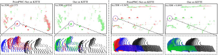
Table I and table II gives the quantitative results of our method evaluated at sfKITTI [13]. The accuracy of our method is substantially ahead of supervised learning methods FlowNet3 [22], FlowNet3D [8], and FLOT [10]. Compared with the self-supervised learning method [9, 23, 11, 25, 24, 28] based on point clouds, learning 3D scene flow on pseudo-LiDAR from real-world images demonstrates an impressive effect. Compared to PointPWC-Net [9], our method improves over 45% on EPE3D, Acc3DS and EPE2D, and improves over 30% on Acc3DR, Outliers and Acc2D, which is a powerful demonstration that Chamfer loss and Laplacian regularization loss can be more effective on pseudo-LiDAR. Our method without fine-tuning still outperforms the results of Mittal et al. (ft) [11] fine-tuning on sfKITTI.
From the bottom of Table I, the 3D scene flow estimator is trained from scratch on a synthesized dataset [12], LiDAR point clouds [20, 14], and real-world stereo/monocular images [20], respectively. It is obvious that self-supervised learning works best on pseudo-LiDAR point clouds estimated from images. This confirms that our method avoids the limitation of estimating the scene flow on the synthesized data set to a certain extent. It also confirms that our method avoids the weakness of learning point motion from LiDAR data. Furthermore, in the last row of Table I, the model trained on FT3D [12] serves as a prior guide for our method. As we have been emphasizing, pseudo-LiDAR point clouds will stimulate the potential of self-supervised loss to a greater extent.
The accuracy of learning 3D scene flow on the 128-beam LiDAR signals [14] is improved compared to the 64-beam LiDAR signals. According to the sentence according to the quantitative results of Table I and Table II, the proposed framework for learning 3D scene flow from pseudo-LiDAR signals still presents greater advantages. To qualitative demonstrate the effectiveness of our method, some visualizations are shown in Fig. 4. Compared to PointPWC-Net [9], the estimated points by our method are mostly correct points on the Acc3DR metric. From the details in Fig. 4, the point clouds estimated from our method overlap well with the ground truth point clouds, confirming the reliability of our method. Finally, the methods in this paper also show excellent perceptual performance in the real world as shown in Figure 5.
| edges | outliers | EPE3D(m) | Acc3DR | EPE2D(px) | |
| 0.2655 | 0.3319 | 11.4530 | |||
| ✓ | 0.1191 | 0.7181 | 5.3741 | ||
| ✓ | ✓ | 0.1156 | 0.7298 | 5.0802 | |
| ✓ | ✓ | ✓ | 0.1103 | 0.7412 | 4.9141 |
| EPE3D() | Acc3DS | EPE2D(px) | ||
| 4 | 2 | 0.1155 | 0.4224 | 5.3325 |
| 8 | 1 | 0.1188 | 0.4044 | 5.3622 |
| 8 | 2 | 0.1103 | 0.4568 | 4.9141 |
| 8 | 4 | 0.1111 | 0.4422 | 4.8438 |
| 16 | 2 | 0.1261 | 0.4237 | 5.5634 |
We test the runtime on a single NVIDIA TITAN RTX GPU. PointPWC-Net takes about 0.1150 seconds on average to perform a training step while our method takes 0.6017 seconds. We consider saving the pseudo-LiDAR point cloud from the depth estimation and enabling the scene flow estimator to learn the scene flow from the saved point cloud. After saving the pseudo-LiDAR signals, the training time is greatly reduced and achieves the same time consumption (about 0.1150 seconds) as PointPWC-Net.
IV-C Ablation Studies
The edge points of the whole scene and the outliers within the scene are the two factors that we focus on. In Table III, the experiments demonstrate that the choice of a suitable scene range and the elimination of outlier points both facilitate the learning of 3D scene flow. In the ablation study, the proposed disparity consistency loss is verified to be very effective for learning 3D scene flow. A point in the point cloud whose distance from its nearest point exceeds a distance threshold is considered as an outlier, where is calculated by Eq. (6). The probability that a point in the point cloud is considered as an outlier is determined by the number of selected points and the standard deviation multiplier threshold . The experiments in Table IV show the best results for elimination of outlier points when is 8 and is 2.
V Conclusion
The method in this paper achieves accurate perception of 3D dynamic scenes on 2D images. The pseudo-LiDAR point cloud is used as a bridge to compensate for the disadvantages of estimating 3D scene flow from LiDAR point clouds. The points in the pseudo-LiDAR point cloud that affect the scene flow estimation are filtered out. In addition, disparity consistency loss was proposed and achieved better self-supervised learning results. The evaluation results demonstrate the advanced performance of our method in the real world datasets.
References
- [1] L. Chen, M. Cui, F. Zhang, B. Hu, and K. Huang, “High-speed scene flow on embedded commercial off-the-shelf systems,” IEEE Transactions on Industrial Informatics, vol. 15, no. 4, pp. 1843–1852, 2018.
- [2] G. Wang, X. Wu, Z. Liu, and H. Wang, “Hierarchical attention learning of scene flow in 3d point clouds,” IEEE Transactions on Image Processing, vol. 30, pp. 5168–5181, 2021.
- [3] S. Wang, Y. Sun, C. Liu, and M. Liu, “Pointtracknet: An end-to-end network for 3-d object detection and tracking from point clouds,” IEEE Robotics and Automation Letters, vol. 5, no. 2, pp. 3206–3212, 2020.
- [4] F. Brickwedde, S. Abraham, and R. Mester, “Mono-sf: Multi-view geometry meets single-view depth for monocular scene flow estimation of dynamic traffic scenes,” in Proceedings of the IEEE/CVF International Conference on Computer Vision, 2019, pp. 2780–2790.
- [5] J. Hur and S. Roth, “Self-supervised multi-frame monocular scene flow,” in Proceedings of the IEEE/CVF Conference on Computer Vision and Pattern Recognition, 2021, pp. 2684–2694.
- [6] Z. Teed and J. Deng, “Raft-3d: Scene flow using rigid-motion embeddings,” in Proceedings of the IEEE/CVF Conference on Computer Vision and Pattern Recognition, 2021, pp. 8375–8384.
- [7] A. Dewan, T. Caselitz, G. D. Tipaldi, and W. Burgard, “Rigid scene flow for 3d lidar scans,” in 2016 IEEE/RSJ International Conference on Intelligent Robots and Systems (IROS), 2016, pp. 1765–1770.
- [8] X. Liu, C. R. Qi, and L. J. Guibas, “Flownet3d: Learning scene flow in 3d point clouds,” in Proceedings of the IEEE/CVF Conference on Computer Vision and Pattern Recognition, 2019, pp. 529–537.
- [9] W. Wu, Z. Y. Wang, Z. Li, W. Liu, and L. Fuxin, “Pointpwc-net: Cost volume on point clouds for (self-) supervised scene flow estimation,” in European Conference on Computer Vision, 2020, pp. 88–107.
- [10] G. Puy, A. Boulch, and R. Marlet, “Flot: Scene flow on point clouds guided by optimal transport,” in ECCV 2020: 16th European Conference, Glasgow, UK, August 23–28, 2020, Proceedings, Part XXVIII 16, 2020, pp. 527–544.
- [11] H. Mittal, B. Okorn, and D. Held, “Just go with the flow: Self-supervised scene flow estimation,” in Proceedings of the IEEE/CVF Conference on Computer Vision and Pattern Recognition, 2020, pp. 11 177–11 185.
- [12] N. Mayer, E. Ilg, P. Hausser, P. Fischer, D. Cremers, A. Dosovitskiy, and T. Brox, “A large dataset to train convolutional networks for disparity, optical flow, and scene flow estimation,” in Proceedings of the IEEE Conference on Computer Vision and Pattern Recognition, 2016, pp. 4040–4048.
- [13] M. Menze, C. Heipke, and A. Geiger, “Object scene flow,” ISPRS Journal of Photogrammetry and Remote Sensing, vol. 140, pp. 60–76, 2018.
- [14] L. Li, K. N. Ismail, H. P. Shum, and T. P. Breckon, “Durlar: A high-fidelity 128-channel lidar dataset with panoramic ambient and reflectivity imagery for multi-modal autonomous driving applications,” in 2021 International Conference on 3D Vision (3DV). IEEE, 2021, pp. 1227–1237.
- [15] Y. Wang, W.-L. Chao, D. Garg, B. Hariharan, M. Campbell, and K. Q. Weinberger, “Pseudo-lidar from visual depth estimation: Bridging the gap in 3d object detection for autonomous driving,” in Proceedings of the IEEE/CVF Conference on Computer Vision and Pattern Recognition (CVPR), June 2019.
- [16] Y. You, Y. Wang, W.-L. Chao, D. Garg, G. Pleiss, B. Hariharan, M. Campbell, and K. Q. Weinberger, “Pseudo-lidar++: Accurate depth for 3d object detection in autonomous driving,” in International Conference on Learning Representations (ICLR), 2020.
- [17] R. Qian, D. Garg, Y. Wang, Y. You, S. Belongie, B. Hariharan, M. Campbell, K. Q. Weinberger, and W.-L. Chao, “End-to-end pseudo-lidar for image-based 3d object detection,” in Proceedings of the IEEE/CVF Conference on Computer Vision and Pattern Recognition, 2020, pp. 5881–5890.
- [18] R. Battrawy, R. Schuster, O. Wasenmüller, Q. Rao, and D. Stricker, “Lidar-flow: Dense scene flow estimation from sparse lidar and stereo images,” in 2019 IEEE/RSJ International Conference on Intelligent Robots and Systems (IROS), 2019, pp. 7762–7769.
- [19] J.-R. Chang and Y.-S. Chen, “Pyramid stereo matching network,” in Proceedings of the IEEE Conference on Computer Vision and Pattern Recognition, 2018, pp. 5410–5418.
- [20] A. Geiger, P. Lenz, C. Stiller, and R. Urtasun, “Vision meets robotics: The kitti dataset,” The International Journal of Robotics Research, vol. 32, no. 11, pp. 1231–1237, 2013.
- [21] J. Bian, Z. Li, N. Wang, H. Zhan, C. Shen, M.-M. Cheng, and I. Reid, “Unsupervised scale-consistent depth and ego-motion learning from monocular video,” Advances in neural information processing systems, vol. 32, 2019.
- [22] E. Ilg, T. Saikia, M. Keuper, and T. Brox, “Occlusions, motion and depth boundaries with a generic network for disparity, optical flow or scene flow estimation,” in Proceedings of the European Conference on Computer Vision (ECCV), 2018, pp. 614–630.
- [23] J. K. Pontes, J. Hays, and S. Lucey, “Scene flow from point clouds with or without learning,” in 2020 International Conference on 3D Vision (3DV), 2020, pp. 261–270.
- [24] R. Li, G. Lin, and L. Xie, “Self-point-flow: Self-supervised scene flow estimation from point clouds with optimal transport and random walk,” in Proceedings of the IEEE/CVF Conference on Computer Vision and Pattern Recognition, 2021, pp. 15 577–15 586.
- [25] G. Wang, C. Jiang, Z. Shen, Y. Miao, and H. Wang, “Sfgan: Unsupervised generative adversarial learning of 3d scene flow from the 3d scene self,” Advanced Intelligent Systems, vol. 4, no. 4, p. 2100197, 2022.
- [26] M.-F. Chang, J. Lambert, P. Sangkloy, J. Singh, S. Bak, A. Hartnett, D. Wang, P. Carr, S. Lucey, D. Ramanan et al., “Argoverse: 3d tracking and forecasting with rich maps,” in Proceedings of the IEEE/CVF Conference on Computer Vision and Pattern Recognition, 2019, pp. 8748–8757.
- [27] H. Caesar, V. Bankiti, A. H. Lang, S. Vora, V. E. Liong, Q. Xu, A. Krishnan, Y. Pan, G. Baldan, and O. Beijbom, “nuscenes: A multimodal dataset for autonomous driving,” in Proceedings of the IEEE/CVF conference on computer vision and pattern recognition, 2020, pp. 11 621–11 631.
- [28] Z. Jin, Y. Lei, N. Akhtar, H. Li, and M. Hayat, “Deformation and correspondence aware unsupervised synthetic-to-real scene flow estimation for point clouds,” in Proceedings of the IEEE/CVF Conference on Computer Vision and Pattern Recognition, 2022, pp. 7233–7243.
- [29] S. F. Bhat, I. Alhashim, and P. Wonka, “Adabins: Depth estimation using adaptive bins,” in Proceedings of the IEEE/CVF Conference on Computer Vision and Pattern Recognition, 2021, pp. 4009–4018.