3D Cinemagraphy from a Single Image
Abstract
We present 3D Cinemagraphy, a new technique that marries 2D image animation with 3D photography. Given a single still image as input, our goal is to generate a video that contains both visual content animation and camera motion. We empirically find that naively combining existing 2D image animation and 3D photography methods leads to obvious artifacts or inconsistent animation. Our key insight is that representing and animating the scene in 3D space offers a natural solution to this task. To this end, we first convert the input image into feature-based layered depth images using predicted depth values, followed by unprojecting them to a feature point cloud. To animate the scene, we perform motion estimation and lift the 2D motion into the 3D scene flow. Finally, to resolve the problem of hole emergence as points move forward, we propose to bidirectionally displace the point cloud as per the scene flow and synthesize novel views by separately projecting them into target image planes and blending the results. Extensive experiments demonstrate the effectiveness of our method. A user study is also conducted to validate the compelling rendering results of our method.
[autoplay,loop,trim = 100 0 0 0,height=]20figures/teaser/holynski-21/059 \animategraphics[autoplay,loop,trim = 50 0 0 0,height=]20figures/teaser/28-mountain/059 \animategraphics[autoplay,loop,trim = 50 0 0 0,height=]20figures/teaser/11-crayon/059 \animategraphics[autoplay,loop,height=]20figures/teaser/24-diffusion/089
1 Introduction
Nowadays, since people can easily take images using smartphone cameras, the number of online photos has increased drastically. However, with the rise of online video-sharing platforms such as YouTube and TikTok, people are no longer content with static images as they have grown accustomed to watching videos. It would be great if we could animate those still images and synthesize videos for a better experience. These living images, termed cinemagraphs, have already been created and gained rapid popularity online [1, 71]. Although cinemagraphs may engage people with the content for longer than a regular photo, they usually fail to deliver an immersive sense of 3D to audiences. This is because cinemagraphs are usually based on a static camera and fail to produce parallax effects. We are therefore motivated to explore ways of animating the photos and moving around the cameras at the same time. As shown in Fig. 1, this will bring many still images to life and provide a drastically vivid experience.
In this paper, we are interested in making the first step towards 3D cinemagraphy that allows both realistic animation of the scene and camera motions with compelling parallax effects from a single image. There are plenty of attempts to tackle either of the two problems. Single-image animation methods [12, 19, 35] manage to produce a realistic animated video from a single image, but they usually operate in 2D space, and therefore they cannot create camera movement effects. Classic novel view synthesis methods [9, 5, 6, 14, 25] and recent implicit neural representations [37, 58, 40] entail densely captured views as input to render unseen camera perspectives. Single-shot novel view synthesis approaches [52, 21, 39, 66] exhibit the potential for generating novel camera trajectories of the scene from a single image. Nonetheless, these methods usually hypothesize that the observed scene is static without moving elements. Directly combining existing state-of-the-art solutions of single-image animation and novel view synthesis yields visual artifacts or inconsistent animation.
To address the above challenges, we present a novel framework that solves the joint task of image animation and novel view synthesis. This framework can be trained to create 3D cinemagraphs from a single still image. Our key intuition is that handling this new task in 3D space would naturally enable both animation and moving cameras simultaneously. With this in mind, we first represent the scene as feature-based layered depth images (LDIs) [50] and unproject the feature LDIs into a feature point cloud. To animate the scene, we perform motion estimation and lift the 2D motion to 3D scene flow using depth values predicted by DPT [45]. Next, we animate the point cloud according to the scene flow. To resolve the problem of hole emergence as points move forward, we are inspired by prior works [19, 3, 38] and propose a 3D symmetric animation technique to bidirectionally displace point clouds, which can effectively fill in those unknown regions. Finally, we synthesize novel views at time by rendering point clouds into target image planes and blending the results. In this manner, our proposed method can automatically create 3D cinemagraphs from a single image. Moreover, our framework is highly extensible, e.g., we can augment our motion estimator with user-defined masks and flow hints for accurate flow estimation and controllable animation.
In summary, our main contributions are:
-
•
We propose a new task of creating 3D cinemagraphs from single images. To this end, we propose a novel framework that jointly learns to solve the task of image animation and novel view synthesis in 3D space.
-
•
We design a 3D symmetric animation technique to address the hole problem as points move forward.
-
•
Our framework is flexible and customized. We can achieve controllable animation by augmenting our motion estimator with user-defined masks and flow hints.
2 Related Work
Single-image animation. Different kinds of methods have been explored to animate still images. Some works [8, 22] focus on animating certain objects via physical simulation but may not be easily applied to more general cases of in-the-wild photos. Given driving videos as guidance, there are plenty of methods that attempt to perform motion transfer on static objects with either a priori knowledge of moving objects [7, 46, 55, 11, 33] or in an unsupervised manner [53, 54, 56]. They entail reference videos to drive the motion of static objects, and thus do not suit our task. Recent advances in generative models have attracted much attention and motivated the community to develop realistic image and video synthesis methods. Many works [51, 34, 69, 32, 31] are based on generative adversarial networks (GANs) and operate transformations in latent space to generate plausible appearance changes and movements. Nonetheless, it is non-trial to allow for explicit control over those latent codes and to animate input imagery in a disentangled manner. As diffusion models [17, 59] improve by leaps and bounds, several diffusion-based works [57, 18, 16] attempt to generate realistic videos from text or images. However, these methods are time-consuming and expensive in terms of computation. Here we focus on methods that utilize learned motion priors to convert a still image into an animated video texture [29, 19, 12, 35, 13]. In particular, Holynski et al. [19] first synthesize the optical flow of the input image via a motion estimation network, then obtain future frames using the estimated flow field. This method renders plausible animation of fluid elements in the input image but suffers from producing camera motions with parallax.
Novel view synthesis from a single image. Novel view synthesis allows for rendering unseen camera perspectives from 2D images and their corresponding camera poses. Recent impressive synthesis results may credit to implicit neural representations [37, 40, 58]. Nevertheless, these methods usually assume dense views as input, which is not always available in most cases. Moreover, they focus on the task of interpolation given multiple views rather than extrapolation. As such, we instead turn to methods aiming at handling single input. Among them, a number of works [72, 62, 63, 26, 70, 15, 28] infer the 3D structure of scenes by learning to predict a scene representation from a single image. These methods are usually trained end-to-end but suffer from generalizing to in-the-wild photos. Most relevant to our work are those approaches [52, 39, 66] that apply depth estimation [45, 67, 68, 65] followed by inpainting occluded regions. For example, 3D Photo [52] estimates monocular depth maps and uses the representation of layered depth images (LDIs) [50, 43], in which context-aware color and depth inpainting are performed. To enable fine-grained detail modeling, SLIDE [21] decomposes the scene into foreground and background via a soft-layering scheme. However, unlike our approach, these methods usually assume the scene is static by default, which largely lessens the sense of reality, especially when some elements such as a creek or smoke are also captured in the input image.
Space-time view synthesis. Space-time view synthesis is the task of rendering novel camera perspectives for dynamic scenes in terms of space and time [30]. Most of the prior works [2, 27, 4] rely on synchronized multi-view videos as input, which prevents their wide applicability. To mitigate this requirement, many neural rendering approaches [30, 41, 44] manage to show promising space-time view synthesis results from monocular videos. They usually train each new scene independently, and thus cannot directly handle in-the-wild inputs. Most related to our work, 3D Moments [64] introduces a novel 3D photography effect where cinematic camera motion and frame interpolation are simultaneously performed. However, this method demands near-duplicate photos as input and is unable to control the animation results. Instead, we show that our method can animate still images while enabling camera motion with 3D parallax. Moreover, we can also extend our system so that users are allowed to interactively control how the photos are animated by providing user-defined masks and flow hints.
3 Method
3.1 Overview
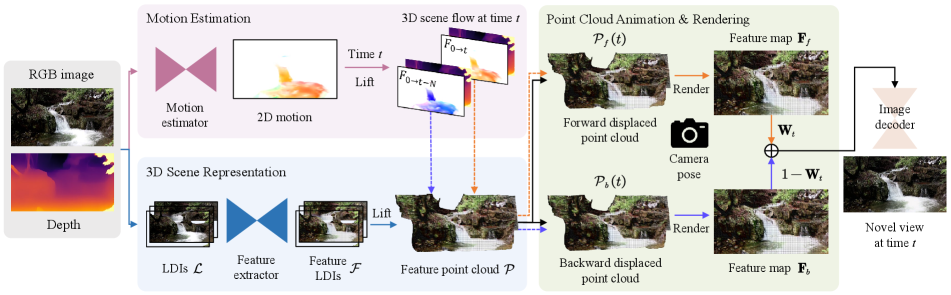
Given a single still image, our goal is to synthesize plausible animation of the scene and simultaneously enable camera motion. The output of our method is a realistic cinemagraph with compelling parallax effects. Fig. 2 schematically illustrates our pipeline. Our method starts by estimating a motion field and a depth map from the input image. We then separate the RGBD input into several layers as per depth discontinuities and inpaint occluded regions, followed by extracting 2D feature maps for each layer, resulting in feature LDIs [50]. To enable scene animation, we lift the 2D motion to 3D scene flow and unproject feature LDIs into a feature point cloud using their corresponding depth values. Thereafter, we bidirectionally animate the point cloud with scene flow using our 3D symmetric animation technique. We end up rendering them into two animated feature maps and composite the results to synthesize novel views at time .
3.2 Motion Estimation
To animate a still image, we wish to estimate the corresponding motion field for the observed scene. Generally, the motion we witness in the real world is extremely complicated as it is time-varying and many events such as occlusion and collision could occur. Intuitively, we could directly adopt prior optical flow estimation methods [60, 61, 20, 10] to accomplish this. However, it is not trivial since they usually take a pair of images as input to compute optical flow. Endo et al. [12] instead propose to learn and predict the motion in a recurrent manner, but this kind of approach is prone to large distortions in the long term. To simplify this, we follow Holynski et al. [19] and assume that a time-invariant and constant-velocity motion field, termed Eulerian flow field, can well approximate the bulk of real-world motions, e.g., water, smoke, and clouds. Formally, we denote as the Eulerian flow field of the scene, which suggests that
| (1) |
where represents the optical flow map from frame to frame . This defines how each pixel in the current frame will move in the future. Specifically, we can obtain the next frame via Euler integration:
| (2) |
where represents the coordinates of a pixel at time . Since the optical flow between consecutive frames is identical, we can easily deduce the displacement field by recursively applying:
| (3) |
where denotes the displacement field from time to time , which describes the course of each pixel in the input image across future frames. To estimate the Eulerian flow field, we adopt an image-to-image translation network as our motion estimator, which is able to map an RGB image to the optical flow.
3.3 3D Scene Representation
One common disadvantage of previous single-image animation methods [29, 19, 12] is that they usually operate in 2D space via a deep image warping technique, which prevents them from creating parallax effects. Instead, to enable camera motion, we propose to lift our workspace into 3D and thus resort to 3D scene representation.
We start by estimating the underlying geometry of the scene using the state-of-the-art monocular depth estimator DPT [45], which can predict reasonable dense depth maps for in-the-wild photos. Following Wang et al. [64], we then convert the RGBD input into an LDI representation [50] by separating it into several layers as per depth discontinuities and inpainting occluded regions. Specifically, we first divide the depth range of the source depth map into multiple intervals using agglomerative clustering [36], followed by creating layered depth images . Next, we inpaint occluded regions of each color and depth layer by applying the pretrained inpainting model from 3D Photo [52]. To improve rendering quality and reduce artifacts, we also introduce a 2D feature extraction network to encode 2D feature maps for each inpainted LDI color layer, resulting in feature LDIs . Finally, in order to enable animation in 3D space, we unproject feature LDIs into 3D via their corresponding inpainted depth layers, yielding a feature point cloud , where and are 3D coordinates and the feature vector for each 3D point respectively.
3.4 Point Cloud Animation and Rendering
We now have the estimated displacement fields and the feature point cloud . Our next step is to animate this point cloud over time. To bridge the gap between 2D displacement fields and 3D scene representation, we first augment the displacement fields with estimated depth values to lift them into 3D scene flow. In other words, we now have a function of time and the coordinates of a 3D point that returns a corresponding 3D translation vector that can shift this 3D point accordingly. Thus, for time , we then move each 3D point by computing its destination as its original position plus a corresponding 3D translation vector, i.e., . Intuitively, this process indeed animates the point cloud from one time to another. However, we empirically find that as points move forward, increasingly large holes emerge. This frequently happens when points leave their original locations without any points filling in those unknown regions.
3D symmetric animation. To resolve this, inspired by prior works [19, 38, 3], we propose a 3D symmetric animation technique that leverages bidirectionally displaced point clouds to complement each other. With 3D symmetric animation, we can borrow textural information from point clouds that move in the opposite direction and integrate both of the animated point clouds to feasibly fill in missing regions. Specifically, we directly replace the original Eulerian flow field with and recursively apply Eq. (3) to generate a reversed displacement field. Similarly, we then lift this 2D displacement field to obtain inverse scene flow, which is employed to produce point clouds with backward movements. As illustrated in Fig. 3, for time , to fill in holes, we respectively apply and to draw associated scene flow fields and use them to move the point cloud, resulting in and , where is the number of frames.

Neural rendering. We now have two bidirectionally animated feature point clouds. Our final step is to render them into animated feature maps and composite the results for synthesizing novel views at time . In particular, given camera poses and intrinsics, we use a differentiable point-based renderer [66] to splat feature point clouds and separately into the target image plane. This process yields 2D feature maps and along with depth maps , and alpha maps , . Next, we wish to fuse and into one feature map . Inspired by prior work [64], our intuition is three-fold: 1) to enable endless and seamless looping, we should assign the weight of the two feature maps based on time so as to guarantee that the first and last frame of the synthesized video are identical; 2) the weight map should favor pixel locations with smaller depth values, in the sense that it is impossible to see objects behind those objects closer to the eye; 3) to avoid missing regions as much as possible, we should greatly increase the contribution of those pixel locations that can fill in holes. With this in mind, we formulate the weight map as follows:
| (4) |
where is the number of frames. Therefore, we can integrate and via:
| (5) |
We also obtain the merged depth map :
| (6) |
Finally, we employ an image decoder network to map the 2D feature map and depth map to a novel view at time . Repeating this method, we are able to synthesize a realistic cinemagraph with compelling parallax effects.
3.5 Training
This section describes our training scheme. In general, we train our image-to-image translation network, 2D feature extraction network, and image decoder network in a two-stage manner.
Training dataset. We use the training set from Holynski et al. [19] as our training dataset. This dataset comprises short video clips of fluid motion that are extracted from longer stock-footage videos. We use the first frames of each video clip and the corresponding ground truth motion fields estimated by a pretrained optical flow network [60] as motion estimation pairs to train our motion estimation network. To develop animation ability, we randomly sample training data from fluid motion video clips. For novel view synthesis training, we require multi-view supervision of the same scene, which is not available in the training set. Instead, we use 3D Photo [52] to generate pseudo ground truth novel views for training.
Two-stage training. Our model is trained in a two-stage manner. Specifically, we first train our motion estimation network using motion estimation pairs. To train the motion estimation network, we minimize GAN loss, GAN feature matching loss [49], and endpoint error as follows:
| (7) |
In the second stage, we freeze the motion estimation network and train the feature extraction network and image decoder network. Our model simultaneously learns to render novel views and animate scenes. For novel view synthesis, we set and use pseudo ground truth novel views to supervise our model. We randomly sample target viewpoints of scenes and require the model to synthesize them. For animation, we train our model on training triplets (start frame, middle frame, end frame) sampled from fluid motion video clips. In particular, we render the middle frame from both directions using and without changing the camera poses and intrinsics. Besides GAN loss and GAN feature matching loss [49], we also enforce VGG perceptual loss [23, 73] and loss between synthesized and ground truth images. The overall loss is as follows:
| (8) |
4 Experiments
4.1 Implementation Details
Our motion estimator is a U-Net [48] based generator with convolutional layers, and we replace Batch Normalization with SPADE [42]. For the feature extraction network and image decoder network, we follow the network architectures from Wang et al. [64]. We adopt the multi-scale discriminator used in SPADE [42] during training.
Our model is trained using the Adam optimizer [24]. We conduct all experiments on a single NVIDIA GeForce RTX 3090 GPU. We train the motion estimation network for around iterations with a batch size of . We set the generator learning rate to and the discriminator learning rate to . For the animation training stage, we train the feature extraction network and image decoder network for around iterations with a learning rate starting at and then decaying exponentially.
4.2 Baselines
In principle, to evaluate our method, we are required to compare it against current state-of-the-art models. However, to our knowledge, we are the first to tackle the novel task of synthesizing a realistic cinemagraph with compelling parallax effects from a single image. As a result, we cannot directly compare to previous works. Instead, we consider forming the following baselines to verify the superiority of our method:
2D animation novel view synthesis. One might consider 2D image animation single-shot novel view synthesis: first employing a 2D image animation method, then a single-shot novel view synthesis method. Specifically, we first adopt a state-of-the-art image animation method [19] to produce an animated looping video. We then apply DPT [45] to estimate geometry and utilize 3D Photo [52] to generate novel views for each frame.
Novel view synthesis 2D animation. It also appears to be feasible that we first render novel views of scenes by 3D Photo [52] and then use the image animation method [19] to animate each viewpoint. Note that motion estimation should be performed for each frame as viewpoints have changed. However, we empirically find that this usually results in varying motion fields across the video. To mitigate this, we further propose using the moving average technique to smooth estimated motions for each frame. This results in novel view synthesis 2D animation + MA.
Naive point cloud animation. Intuitively, we may also consider directly unprojecting pixels into 3D space and subsequently moving and rendering the RGB point cloud. Specifically, given a single input image, we first predict the depth map using DPT [45] and estimate 2D optical flow. We then lift the pixels and optical flow into 3D space to form RGB point clouds and scene flow. Finally, we animate RGB point clouds over time according to the scene flow and project these point clouds into target viewpoints. This baseline also faces a similar issue: as time goes by, large holes gradually appear. One might also employ our 3D symmetric animation technique to further enhance this baseline, i.e., naive point cloud animation + 3DSA.
4.3 Results


Evaluation dataset. Since Holynski et al. [19] only provide a single image for each scene in the test set, we use the validation set from Holynski et al. [19] to evaluate our method and baselines. The validation set consists of unique scenes with samples of ground truth video clips captured by static cameras.
Experimental setup. For evaluation, we render novel views of the ground truth videos in different trajectories, resulting in ground truth frames for each sample. This process does not involve inpainting, thus ground truth frames may contain holes. Only considering valid pixels when calculating metrics, we compare the predicted images with the ground truth frames at the same time and viewpoint. For a fair comparison, all methods utilize the depth maps estimated by DPT [45]. Since we focus on comparing rendering quality, all methods use ground truth optical flows, except that NVS [52] 2D Anim. [19] and NVS [52] 2D Anim. [19] + MA have to estimate optical flows for each frame apart from the first frame. We adopt PSNR, SSIM, and LPIPS [73] as our evaluation metrics.
Quantitative comparisons. As shown in Table 1, our method outperforms all baselines across all metrics by a large margin. This result implies that our method achieves better perceptual quality and produces more realistic renderings, which demonstrates the superiority and effectiveness of our method.
Qualitative comparisons. We showcase the visual comparisons in Fig. 4. One can observe that our method presents photorealistic results while other comparative baselines produce more or less visual artifacts. 2D Anim. [19] NVS [52] intends to generate stripped flickering artifacts. This is because 2D Anim. [19] NVS [52] predicts the depth map for each animated frame, leading to frequent changes in the 3D structure of the scene and inconsistent inpainting. NVS [52] 2D Anim. [19] and NVS [52] 2D Anim. [19] + MA show jelly-like effects as optical flow should be estimated for each novel view. This results in varying motion fields across the video and thus inconsistent animation. Although Naive PC Anim. and Naive PC Anim. + 3DSA also lift the workspace into 3D, they are often prone to produce noticeable holes inevitably. One reason for this is that they do not perform inpainting. Note that some artifacts are difficult to observe when only scanning static figures.
| Comparison | Human preference |
| 2D Anim. [19] NVS [52] / Ours | 12.5% / 87.5% |
| NVS [52] 2D Anim. [19] / Ours | 3.9% / 96.1% |
| NVS [52] 2D Anim. [19] + MA / Ours | 6.1% / 93.9% |
| Naive PC Anim. / Ours | 7.6% / 92.4% |
| Naive PC Anim. + 3DSA / Ours | 8.6% / 91.4% |
| 3D Photo [52] / Ours | 10.5% / 89.5% |
| Holynski et al. [19] / Ours | 29.9% / 70.1% |
| PSNR | SSIM | LPIPS | |
| w/o features | 21.50 | 0.674 | 0.228 |
| w/o inpainting | 22.86 | 0.763 | 0.216 |
| w/o 3D symmetric animation | 22.99 | 0.768 | 0.199 |
| Full model | 23.33 | 0.776 | 0.197 |
Controllable animation. Our method is able to create 3D cinemagraphs from a single image automatically. Further, we show that our framework is also highly extensible. For example, we can involve masks and flow hints as extra inputs to augment our motion estimator. This brings two advantages: (1) more accurate flow estimation; (2) interactive and controllable animation. As shown in Fig. 5, we can control the animation of the scene by providing various masks and motion hints to obtain different motion fields.
Generalizing on in-the-wild photos. To further demonstrate the generalization of our method, we also test our method on in-the-wild photos. We first create cinemagraphs with camera motions on the test set from Holynski et al. [19], where, for each scene, only a single image is provided. We then select some online images at random to test our method. To accurately estimate motion fields, we provide masks and flow hints as extra inputs to our motion estimator. As shown in Fig. 6, our method produces reasonable results for in-the-wild inputs while other comparative alternatives yield visual artifacts or inconsistent animation.

4.4 User Study
We further conduct a user study to investigate how our method performs in the view of humans when compared with all baselines, 3D Photo [52], and Holynski et al. [19]. Specifically, we collect photos from the test set of Holynski et al. [19] and the Internet. We use different approaches to generate videos with identical settings. During the study, we show each participant an input image and two animated videos generated by our method and a randomly selected approach in random order. volunteers are invited to choose the method with better perceptual quality and realism, or none if it is hard to judge. We report the results in Table 2, which points out that our method surpasses alternative methods by a large margin in terms of the sense of reality and immersion.
4.5 Ablation Study
To validate the effect of each component, we conduct an ablation study on the validation set from Holynski et al. [19] and show the results in Table 3. One can observe: i) 3D symmetric animation technique matters because it allows us to leverage bidirectionally displaced point clouds to complement each other and feasibly fill in missing regions; ii) introducing inpainting when constructing 3D geometry can improve the performance as this allows our model to produce plausible structures around depth discontinuities and fill in holes; iii) switching from directly using RGB colors to features in 3D scene representation significantly improves the rendering quality and reduces artifacts.
5 Conclusion
In this paper, we introduce a novel task of creating 3D cinemagraphs from single images. To this end, we present a simple yet effective method that makes a connection between image animation and novel view synthesis. We show that our method produces plausible animation of the scene while allowing camera movements. Our framework is flexible and customized. For accurate motion estimation and controllable animation, we can further include masks and flow hints as extra input for the motion estimator. Therefore, users can control how the scene is animated. Furthermore, our method generalizes well to in-the-wild photos, even like paintings or synthetic images generated by diffusion models. We conduct extensive experiments to verify the effectiveness and superiority of our method. A user study also demonstrates that our method generates realistic 3D cinemagraphs. We hope that our work can bring 3D cinemagraphy into the sight of a broader community and motivate further research.
Limitations and future work. Our method may not work well when the depth prediction module estimates erroneous geometry from the input image, e.g., thin structures. In addition, inappropriate motion fields will sometimes lead to undesirable results, e.g., some regions are mistakenly identified as frozen. As we take the first step towards 3D cinemagraphy, in this paper, we focus on handling common moving elements, i.e., fluids. In other words, our method may not apply to more complex motions, e.g., cyclic motion. We leave this for our future work.
Acknowledgements. This study is supported under the RIE2020 Industry Alignment Fund – Industry Collaboration Projects (IAF-ICP) Funding Initiative, as well as cash and in-kind contribution from the industry partner(s). This work is also supported by Adobe Gift and the Ministry of Education, Singapore, under its Academic Research Fund Tier 2 (MOE-T2EP20220-0007) and Tier 1 (RG14/22).
References
- [1] Jiamin Bai, Aseem Agarwala, Maneesh Agrawala, and Ravi Ramamoorthi. Automatic cinemagraph portraits. In Computer Graphics Forum, volume 32, pages 17–25. Wiley Online Library, 2013.
- [2] Aayush Bansal, Minh Vo, Yaser Sheikh, Deva Ramanan, and Srinivasa Narasimhan. 4d visualization of dynamic events from unconstrained multi-view videos. In Proceedings of the IEEE/CVF Conference on Computer Vision and Pattern Recognition (CVPR), pages 5366–5375, 2020.
- [3] Wenbo Bao, Wei-Sheng Lai, Chao Ma, Xiaoyun Zhang, Zhiyong Gao, and Ming-Hsuan Yang. Depth-aware video frame interpolation. In Proceedings of the IEEE/CVF Conference on Computer Vision and Pattern Recognition (CVPR), pages 3703–3712, 2019.
- [4] Mojtaba Bemana, Karol Myszkowski, Hans-Peter Seidel, and Tobias Ritschel. X-Fields: Implicit neural view-, light-and time-image interpolation. ACM Transactions on Graphics (TOG), 39(6):1–15, 2020.
- [5] Chris Buehler, Michael Bosse, Leonard McMillan, Steven Gortler, and Michael Cohen. Unstructured lumigraph rendering. In Proceedings of the 28th annual conference on Computer graphics and interactive techniques, pages 425–432, 2001.
- [6] Jin-Xiang Chai, Xin Tong, Shing-Chow Chan, and Heung-Yeung Shum. Plenoptic sampling. In Proceedings of the 27th annual conference on Computer graphics and interactive techniques, pages 307–318, 2000.
- [7] Caroline Chan, Shiry Ginosar, Tinghui Zhou, and Alexei A Efros. Everybody dance now. In Proceedings of the IEEE/CVF International Conference on Computer Vision (ICCV), pages 5933–5942, 2019.
- [8] Yung-Yu Chuang, Dan B Goldman, Ke Colin Zheng, Brian Curless, David H Salesin, and Richard Szeliski. Animating pictures with stochastic motion textures. ACM Transactions on Graphics (TOG), 24(3):853–860, 2005.
- [9] Paul E Debevec, Camillo J Taylor, and Jitendra Malik. Modeling and rendering architecture from photographs: A hybrid geometry-and image-based approach. In Proceedings of the 23rd annual conference on Computer graphics and interactive techniques, pages 11–20, 1996.
- [10] Alexey Dosovitskiy, Philipp Fischer, Eddy Ilg, Philip Hausser, Caner Hazirbas, Vladimir Golkov, Patrick Van Der Smagt, Daniel Cremers, and Thomas Brox. FlowNet: Learning optical flow with convolutional networks. In Proceedings of the IEEE/CVF International Conference on Computer Vision (ICCV), pages 2758–2766, 2015.
- [11] Michail Christos Doukas, Stefanos Zafeiriou, and Viktoriia Sharmanska. HeadGAN: One-shot neural head synthesis and editing. In Proceedings of the IEEE/CVF International Conference on Computer Vision (ICCV), pages 14398–14407, 2021.
- [12] Yuki Endo, Yoshihiro Kanamori, and Shigeru Kuriyama. Animating Landscape: Self-supervised learning of decoupled motion and appearance for single-image video synthesis. ACM Transactions on Graphics (Proceedings of ACM SIGGRAPH Asia 2019), 38(6):175:1–175:19, 2019.
- [13] Siming Fan, Jingtan Piao, Chen Qian, Kwan-Yee Lin, and Hongsheng Li. Simulating fluids in real-world still images. arXiv preprint arXiv:2204.11335, 2022.
- [14] Steven J Gortler, Radek Grzeszczuk, Richard Szeliski, and Michael F Cohen. The lumigraph. In Proceedings of the 23rd annual conference on Computer graphics and interactive techniques, pages 43–54, 1996.
- [15] Yuxuan Han, Ruicheng Wang, and Jiaolong Yang. Single-view view synthesis in the wild with learned adaptive multiplane images. In ACM SIGGRAPH 2022 Conference Proceedings, pages 1–8, 2022.
- [16] Jonathan Ho, William Chan, Chitwan Saharia, Jay Whang, Ruiqi Gao, Alexey Gritsenko, Diederik P Kingma, Ben Poole, Mohammad Norouzi, David J Fleet, et al. Imagen Video: High definition video generation with diffusion models. arXiv preprint arXiv:2210.02303, 2022.
- [17] Jonathan Ho, Ajay Jain, and Pieter Abbeel. Denoising diffusion probabilistic models. In Advances in Neural Information Processing Systems (NeurIPS), 2020.
- [18] Jonathan Ho, Tim Salimans, Alexey Gritsenko, William Chan, Mohammad Norouzi, and David J Fleet. Video diffusion models. arXiv preprint arXiv:2204.03458, 2022.
- [19] Aleksander Holynski, Brian L. Curless, Steven M. Seitz, and Richard Szeliski. Animating pictures with eulerian motion fields. In Proceedings of the IEEE/CVF Conference on Computer Vision and Pattern Recognition (CVPR), pages 5810–5819, 2021.
- [20] Eddy Ilg, Nikolaus Mayer, Tonmoy Saikia, Margret Keuper, Alexey Dosovitskiy, and Thomas Brox. FlowNet 2.0: Evolution of optical flow estimation with deep networks. In Proceedings of the IEEE/CVF Conference on Computer Vision and Pattern Recognition (CVPR), pages 2462–2470, 2017.
- [21] Varun Jampani, Huiwen Chang, Kyle Sargent, Abhishek Kar, Richard Tucker, Michael Krainin, Dominik Kaeser, William T Freeman, David Salesin, Brian Curless, and Ce Liu. SLIDE: Single image 3d photography with soft layering and depth-aware inpainting. In Proceedings of the IEEE/CVF International Conference on Computer Vision (ICCV), 2021.
- [22] Wei-Cih Jhou and Wen-Huang Cheng. Animating still landscape photographs through cloud motion creation. IEEE Transactions on Multimedia, 18(1):4–13, 2015.
- [23] Justin Johnson, Alexandre Alahi, and Li Fei-Fei. Perceptual losses for real-time style transfer and super-resolution. In Proceedings of the European Conference on Computer Vision (ECCV), pages 694–711. Springer, 2016.
- [24] Diederik P Kingma and Jimmy Ba. Adam: A method for stochastic optimization. arXiv preprint arXiv:1412.6980, 2014.
- [25] Marc Levoy and Pat Hanrahan. Light field rendering. In Proceedings of the 23rd annual conference on Computer graphics and interactive techniques, pages 31–42, 1996.
- [26] Jiaxin Li, Zijian Feng, Qi She, Henghui Ding, Changhu Wang, and Gim Hee Lee. MINE: Towards continuous depth mpi with nerf for novel view synthesis. In Proceedings of the IEEE/CVF Conference on Computer Vision and Pattern Recognition (CVPR), pages 12578–12588, 2021.
- [27] Tianye Li, Mira Slavcheva, Michael Zollhoefer, Simon Green, Christoph Lassner, Changil Kim, Tanner Schmidt, Steven Lovegrove, Michael Goesele, Richard Newcombe, et al. Neural 3d video synthesis from multi-view video. In Proceedings of the IEEE/CVF Conference on Computer Vision and Pattern Recognition (CVPR), pages 5521–5531, 2022.
- [28] Xingyi Li, Chaoyi Hong, Yiran Wang, Zhiguo Cao, Ke Xian, and Guosheng Lin. Symmnerf: Learning to explore symmetry prior for single-view view synthesis. In Proceedings of the Asian Conference on Computer Vision (ACCV), pages 1726–1742, 2022.
- [29] Yijun Li, Chen Fang, Jimei Yang, Zhaowen Wang, Xin Lu, and Ming-Hsuan Yang. Flow-grounded spatial-temporal video prediction from still images. In Proceedings of the European Conference on Computer Vision (ECCV), pages 600–615, 2018.
- [30] Zhengqi Li, Simon Niklaus, Noah Snavely, and Oliver Wang. Neural scene flow fields for space-time view synthesis of dynamic scenes. In Proceedings of the IEEE/CVF Conference on Computer Vision and Pattern Recognition (CVPR), pages 6498–6508, 2021.
- [31] Chieh Hubert Lin, Yen-Chi Cheng, Hsin-Ying Lee, Sergey Tulyakov, and Ming-Hsuan Yang. InfinityGAN: Towards infinite-pixel image synthesis. In International Conference on Learning Representations (ICLR), 2022.
- [32] Andrew Liu, Richard Tucker, Varun Jampani, Ameesh Makadia, Noah Snavely, and Angjoo Kanazawa. Infinite nature: Perpetual view generation of natural scenes from a single image. In Proceedings of the IEEE/CVF International Conference on Computer Vision (ICCV), pages 14458–14467, 2021.
- [33] Wen Liu, Zhixin Piao, Jie Min, Wenhan Luo, Lin Ma, and Shenghua Gao. Liquid Warping GAN: A unified framework for human motion imitation, appearance transfer and novel view synthesis. In Proceedings of the IEEE/CVF International Conference on Computer Vision (ICCV), pages 5904–5913, 2019.
- [34] Elizaveta Logacheva, Roman Suvorov, Oleg Khomenko, Anton Mashikhin, and Victor Lempitsky. DeepLandscape: Adversarial modeling of landscape videos. In Proceedings of the European Conference on Computer Vision (ECCV), pages 256–272. Springer, 2020.
- [35] Aniruddha Mahapatra and Kuldeep Kulkarni. Controllable animation of fluid elements in still images. In Proceedings of the IEEE/CVF Conference on Computer Vision and Pattern Recognition (CVPR), pages 3667–3676, 2022.
- [36] Oded Maimon and Lior Rokach. Data mining and knowledge discovery handbook. 2005.
- [37] Ben Mildenhall, Pratul P. Srinivasan, Matthew Tancik, Jonathan T. Barron, Ravi Ramamoorthi, and Ren Ng. NeRF: Representing scenes as neural radiance fields for view synthesis. In Proceedings of the European Conference on Computer Vision (ECCV), 2020.
- [38] Simon Niklaus and Feng Liu. Softmax splatting for video frame interpolation. In Proceedings of the IEEE/CVF Conference on Computer Vision and Pattern Recognition (CVPR), pages 5437–5446, 2020.
- [39] Simon Niklaus, Long Mai, Jimei Yang, and Feng Liu. 3d ken burns effect from a single image. ACM Transactions on Graphics (ToG), 38(6):1–15, 2019.
- [40] Jeong Joon Park, Peter Florence, Julian Straub, Richard Newcombe, and Steven Lovegrove. DeepSDF: Learning continuous signed distance functions for shape representation. In Proceedings of the IEEE/CVF Conference on Computer Vision and Pattern Recognition (CVPR), pages 165–174, 2019.
- [41] Keunhong Park, Utkarsh Sinha, Jonathan T Barron, Sofien Bouaziz, Dan B Goldman, Steven M Seitz, and Ricardo Martin-Brualla. Nerfies: Deformable neural radiance fields. In Proceedings of the IEEE/CVF International Conference on Computer Vision (ICCV), pages 5865–5874, 2021.
- [42] Taesung Park, Ming-Yu Liu, Ting-Chun Wang, and Jun-Yan Zhu. Semantic image synthesis with spatially-adaptive normalization. In Proceedings of the IEEE/CVF Conference on Computer Vision and Pattern Recognition (CVPR), pages 2337–2346, 2019.
- [43] Juewen Peng, Jianming Zhang, Xianrui Luo, Hao Lu, Ke Xian, and Zhiguo Cao. Mpib: An mpi-based bokeh rendering framework for realistic partial occlusion effects. In Proceedings of the European Conference on Computer Vision (ECCV), pages 590–607. Springer, 2022.
- [44] Albert Pumarola, Enric Corona, Gerard Pons-Moll, and Francesc Moreno-Noguer. D-NeRF: Neural radiance fields for dynamic scenes. In Proceedings of the IEEE/CVF Conference on Computer Vision and Pattern Recognition (CVPR), pages 10318–10327, 2021.
- [45] René Ranftl, Alexey Bochkovskiy, and Vladlen Koltun. Vision transformers for dense prediction. In Proceedings of the IEEE/CVF International Conference on Computer Vision (ICCV), pages 12179–12188, 2021.
- [46] Yurui Ren, Xiaoming Yu, Junming Chen, Thomas H Li, and Ge Li. Deep image spatial transformation for person image generation. In Proceedings of the IEEE/CVF Conference on Computer Vision and Pattern Recognition (CVPR), pages 7690–7699, 2020.
- [47] Robin Rombach, Andreas Blattmann, Dominik Lorenz, Patrick Esser, and Björn Ommer. High-resolution image synthesis with latent diffusion models. In Proceedings of the IEEE/CVF Conference on Computer Vision and Pattern Recognition (CVPR), pages 10684–10695, 2022.
- [48] Olaf Ronneberger, Philipp Fischer, and Thomas Brox. U-Net: Convolutional networks for biomedical image segmentation. In International Conference on Medical Image Computing and Computer Assisted Intervention (MICCAI), pages 234–241. Springer, 2015.
- [49] Tim Salimans, Ian Goodfellow, Wojciech Zaremba, Vicki Cheung, Alec Radford, and Xi Chen. Improved techniques for training gans. In Advances in Neural Information Processing Systems (NeurIPS), 2016.
- [50] Jonathan Shade, Steven Gortler, Li-wei He, and Richard Szeliski. Layered depth images. In Proceedings of the 25th annual conference on Computer graphics and interactive techniques, pages 231–242, 1998.
- [51] Tamar Rott Shaham, Tali Dekel, and Tomer Michaeli. SinGAN: Learning a generative model from a single natural image. In Proceedings of the IEEE/CVF International Conference on Computer Vision (ICCV), pages 4570–4580, 2019.
- [52] Meng-Li Shih, Shih-Yang Su, Johannes Kopf, and Jia-Bin Huang. 3d photography using context-aware layered depth inpainting. In Proceedings of the IEEE/CVF Conference on Computer Vision and Pattern Recognition (CVPR), 2020.
- [53] Aliaksandr Siarohin, Stéphane Lathuilière, Sergey Tulyakov, Elisa Ricci, and Nicu Sebe. Animating arbitrary objects via deep motion transfer. In Proceedings of the IEEE/CVF Conference on Computer Vision and Pattern Recognition (CVPR), pages 2377–2386, 2019.
- [54] Aliaksandr Siarohin, Stéphane Lathuilière, Sergey Tulyakov, Elisa Ricci, and Nicu Sebe. First order motion model for image animation. In Advances in Neural Information Processing Systems (NeurIPS), 2019.
- [55] Aliaksandr Siarohin, Enver Sangineto, Stéphane Lathuiliere, and Nicu Sebe. Deformable gans for pose-based human image generation. In Proceedings of the IEEE/CVF Conference on Computer Vision and Pattern Recognition (CVPR), pages 3408–3416, 2018.
- [56] Aliaksandr Siarohin, Oliver J Woodford, Jian Ren, Menglei Chai, and Sergey Tulyakov. Motion representations for articulated animation. In Proceedings of the IEEE/CVF Conference on Computer Vision and Pattern Recognition (CVPR), pages 13653–13662, 2021.
- [57] Uriel Singer, Adam Polyak, Thomas Hayes, Xi Yin, Jie An, Songyang Zhang, Qiyuan Hu, Harry Yang, Oron Ashual, Oran Gafni, et al. Make-A-Video: Text-to-video generation without text-video data. arXiv preprint arXiv:2209.14792, 2022.
- [58] Vincent Sitzmann, Michael Zollhoefer, and Gordon Wetzstein. Scene Representation Networks: Continuous 3d-structure-aware neural scene representations. In Advances in Neural Information Processing Systems (NeurIPS), 2019.
- [59] Jascha Sohl-Dickstein, Eric Weiss, Niru Maheswaranathan, and Surya Ganguli. Deep unsupervised learning using nonequilibrium thermodynamics. In International Conference on Machine Learning (ICML), pages 2256–2265. PMLR, 2015.
- [60] Deqing Sun, Xiaodong Yang, Ming-Yu Liu, and Jan Kautz. PWC-Net: Cnns for optical flow using pyramid, warping, and cost volume. In Proceedings of the IEEE conference on computer vision and pattern recognition, pages 8934–8943, 2018.
- [61] Zachary Teed and Jia Deng. RAFT: Recurrent all-pairs field transforms for optical flow. In Proceedings of the European Conference on Computer Vision (ECCV), pages 402–419, 2020.
- [62] Richard Tucker and Noah Snavely. Single-view view synthesis with multiplane images. In Proceedings of the IEEE/CVF Conference on Computer Vision and Pattern Recognition (CVPR), pages 551–560, 2020.
- [63] Shubham Tulsiani, Richard Tucker, and Noah Snavely. Layer-structured 3d scene inference via view synthesis. In Proceedings of the European Conference on Computer Vision (ECCV), pages 302–317, 2018.
- [64] Qianqian Wang, Zhengqi Li, David Salesin, Noah Snavely, Brian Curless, and Janne Kontkanen. 3d moments from near-duplicate photos. In Proceedings of the IEEE/CVF Conference on Computer Vision and Pattern Recognition (CVPR), 2022.
- [65] Yiran Wang, Zhiyu Pan, Xingyi Li, Zhiguo Cao, Ke Xian, and Jianming Zhang. Less is more: Consistent video depth estimation with masked frames modeling. In Proceedings of the 30th ACM International Conference on Multimedia (ACM MM), pages 6347–6358, 2022.
- [66] Olivia Wiles, Georgia Gkioxari, Richard Szeliski, and Justin Johnson. SynSin: End-to-end view synthesis from a single image. In Proceedings of the IEEE/CVF Conference on Computer Vision and Pattern Recognition (CVPR), pages 7467–7477, 2020.
- [67] Ke Xian, Chunhua Shen, Zhiguo Cao, Hao Lu, Yang Xiao, Ruibo Li, and Zhenbo Luo. Monocular relative depth perception with web stereo data supervision. In Proceedings of the IEEE/CVF Conference on Computer Vision and Pattern Recognition (CVPR), pages 311–320, 2018.
- [68] Ke Xian, Jianming Zhang, Oliver Wang, Long Mai, Zhe Lin, and Zhiguo Cao. Structure-guided ranking loss for single image depth prediction. In Proceedings of the IEEE/CVF Conference on Computer Vision and Pattern Recognition (CVPR), pages 611–620, 2020.
- [69] Wei Xiong, Wenhan Luo, Lin Ma, Wei Liu, and Jiebo Luo. Learning to generate time-lapse videos using multi-stage dynamic generative adversarial networks. In Proceedings of the IEEE/CVF Conference on Computer Vision and Pattern Recognition (CVPR), pages 2364–2373, 2018.
- [70] Dejia Xu, Yifan Jiang, Peihao Wang, Zhiwen Fan, Humphrey Shi, and Zhangyang Wang. SinNeRF: Training neural radiance fields on complex scenes from a single image. In Proceedings of the European Conference on Computer Vision (ECCV), pages 736–753. Springer, 2022.
- [71] Hang Yan, Yebin Liu, and Yasutaka Furukawa. Turning an urban scene video into a cinemagraph. In Proceedings of the IEEE/CVF Conference on Computer Vision and Pattern Recognition (CVPR), pages 394–402, 2017.
- [72] Alex Yu, Vickie Ye, Matthew Tancik, and Angjoo Kanazawa. pixelNeRF: Neural radiance fields from one or few images. In Proceedings of the IEEE/CVF Conference on Computer Vision and Pattern Recognition (CVPR), pages 4578–4587, 2021.
- [73] Richard Zhang, Phillip Isola, Alexei A Efros, Eli Shechtman, and Oliver Wang. The unreasonable effectiveness of deep features as a perceptual metric. In Proceedings of the IEEE/CVF Conference on Computer Vision and Pattern Recognition (CVPR), pages 586–595, 2018.