2D-Shapley: A Framework for Fragmented Data Valuation
2D-Shapley: A Framework for Fragmented Data Valuation
Supplementary Materials
Abstract
Data valuation—quantifying the contribution of individual data sources to certain predictive behaviors of a model—is of great importance to enhancing the transparency of machine learning and designing incentive systems for data sharing. Existing work has focused on evaluating data sources with the shared feature or sample space. How to valuate fragmented data sources of which each only contains partial features and samples remains an open question. We start by presenting a method to calculate the counterfactual of removing a fragment from the aggregated data matrix. Based on the counterfactual calculation, we further propose 2D-Shapley, a theoretical framework for fragmented data valuation that uniquely satisfies some appealing axioms in the fragmented data context. 2D-Shapley empowers a range of new use cases, such as selecting useful data fragments, providing interpretation for sample-wise data values, and fine-grained data issue diagnosis.
1 Introduction
Data are essential ingredients for building machine learning (ML) applications. The ability to quantify and measure the value of data is crucial to the entire lifecycle of ML: from cleaning poor-quality samples and tracking important ones to be collected during data preparation to setting proper proprieties over samples during training to interpret why certain behaviors of a model emerge during deployment. Determining the value of data is also central to designing incentive systems for data sharing and implementing current policies about the monetarization of personal data.

Current literature of data valuation (Jia et al., 2019b; Ghorbani & Zou, 2019) has exclusively focused on valuing horizontally partitioned data—in other words, each data source to be valued shares the same feature space. How to value vertically partitioned data, where each data source provides a different feature but shares the same sample space, has been studied in the context of ML interpretability (Covert et al., 2020). However, none of these abstractions could fully capture the complexity of real-world scenarios, where data sources can have non-overlapping features and samples (termed as fragmented data sources hereinafter).
Example 1.
Consider two banks, and , and two e-commerce companies, and , located in Region and . These four institutions are interested in collaboratively building an ML model to predict users’ credit scores with their data. Due to the geographical difference, and have a different user group from and . Also, due to the difference in business, and provide different features than what and can offer. Overall, the four institutions partition the aggregated data horizontally and vertically, as illustrated by Figure 1(c). How to quantify each institution’s contribution to the joint model training?
Example 2.
Due to inevitable errors occurring during the data generation and collection processes, real-world data are seldom high quality. Suppose that a data analyst is interested in identifying some potentially erroneous entries in a dataset. Existing horizontal and vertical data valuation tools can help locate the rows or columns that could contain errors by returning the ones with the lowest values. Nevertheless, can we perform more fine-grained detection—e.g., how to pinpoint the coordinate of erroneous entries?
Example 3.
Horizontal data valuation is now widely used to explain the importance of each sample to a learning outcome (Tang et al., 2021; Karlaš et al., 2022). But how can a data analyst further explain these sample importance scores—why a sample receives a certain importance score? Is a sample “low-quality” because it contains several “moderate low quality” features or an “exceptionally low quality” feature?
Answering the above questions calls for a quantitative understanding of how each block in the data matrix (e.g. a sub-matrix as in Ex. 1 or a single entry as in Ex. 2 and 3) contributes to the outcome of learning.
Technical Challenges. The problem of block valuation requires rethinking about fundamental aspects of data valuation. Existing data valuation theory consists of two basic modules at a conceptual level: (1) Counterfactual Analysis, where one calculates how the utility of a subset of data sources would change after the source to be valued is removed; and (2) Fair Attribution, where a data source is valued based on a weighted average of its marginal utilities for different subsets and the weights are set for the value to satisfy certain fairness properties. The fairness notion considered by the past valuation schemes requires that permuting the order of different data sources does not change their value.
For horizontal and vertical valuation, the counterfactual can be simply calculated by taking the difference between the model performance trained on a subset of columns or rows and the performance with one column or row being removed. However, it is unclear how to calculate the counterfactual when a block is excluded because the remaining data matrix could be incomplete. Besides, the fairness notion of existing data value notions is no longer appropriate in the context of block valuation. As a concrete example to illustrate this point, consider Figure 1(c) and suppose the two blocks on the left provide temperature measurements as features and the ones on the right are humidity measurements. In this case, one should not expect the value to be unchanged when two blocks with different physical meanings (e.g., yellow and pink) are swapped.
Contributions. This paper presents the first focused study on data valuation without assuming shared feature space or sample space. Toward that end, we make the following contributions.
-
•
We present an approach that enables evaluation of the marginal contribution of a block within the data matrix to any other block with non-overlapping sample and feature spaces.
-
•
We abstract the block valuation problem into a two-dimensional (2D) cooperative game, where the utility function is invariant to column permutations and row permutations but not to any arbitrary entry permutations.
-
•
We propose axioms that a proper valuation scheme should satisfy in the 2D game and show that the axioms lead to a unique representation of the value assignment (referred to as 2D-Shapley). Particularly, this representation is a natural generalization of the Shapley value (Shapley, 1997)—a celebrated value attribution scheme widely used in data valuation among other applications.
-
•
We demonstrate that 2D-Shapley enables new applications, including selecting useful data fragments, providing interpretation for sample-wise data values, and fine-grained data issue diagnosis.
2 Background and Related Work
In a typical setting, a set of data sources are used to learn an ML model, which achieves a certain performance score. The goal of data valuation is to quantify the contribution of each data source toward achieving the performance score. The definition of a data source depends on the context in which the data valuation results are utilized. For instance, when using data valuation to interpret how the global behavior of the ML model depends on individual samples or individual features, a sample or a feature in the training data is regarded as a data source; when using data valuation to inform the reward design for data sharing, the collection of all samples or all features contributed by the same entities is regarded as a data source.
Formally, let denotes the index set of training data sources. A data valuation scheme assigns a score to each training data source in a way that reflects their contribution. These scores are referred to as data values. To analyze a source’s “contribution”, we define a utility function , which maps any subset of the data sources to a score indicating the usefulness of the subset. represents the power set of , i.e., the set of all subsets of , including the empty set and itself. For the classification task, a common choice for is the performance of a model trained on the input subset, i.e., , where is a learning algorithm that takes a set of sources as input and returns a model, and acc is a metric function to evaluate the performance of a given model, e.g., the accuracy of a model on a hold-out validation set.
Past research has proposed various ways to characterize data values given the utility function, among which the Shapley value is arguably the most widely used scheme for data valuation. The Shapley value is defined as
|
|
(1) |
To differentiate from the proposed work, we will refer to the Shapley value defined in Eq. (1) as 1D-Shapley. 1D-Shapley is popular due to its unique satisfaction of the following four axioms (Shapley, 1953):
-
Dummy: if for any and some , then .
-
Symmetry: let be any permutation of and , then .
-
Linearity: For utility functions and any , .
-
Efficiency: for every .
The symmetry axiom embodies fairness. In particular, arises upon the reindexing of data sources with the indices ; the symmetry axiom states that the evaluation of a particular position should not depend on the indices of the data sources.
Although the Shapley value was justified through these axioms in prior literature, the necessity of each axiom depends on the actual use case of data valuation results. Recent literature has studied new data value notions obtained by relaxing some of the aforementioned axioms and enabled improvements in terms of accuracy of bad data identification (Kwon & Zou, 2022), robustness to learning stochasticity (Wang & Jia, 2023; Wu et al., 2022a), and computational efficiency (Yan & Procaccia, 2021). For instance, relaxing the efficiency axiom gives rise to semi-values (Kwon & Zou, 2022; Wang & Jia, 2023); relaxing the linearity axiom gives rise to least cores (Yan & Procaccia, 2021). This paper will focus on generalizing 1D-Shapley to block valuation. As we will expound on later, 1D-Shapley faces two limitations to serve a reasonable notion for block-wise values. Note that 1D-Shapley and the aforementioned relaxed notions share a similar structure: all of them are based on the marginal utility of a data source. Hence, our effort to generalize the 1D-Shapley to new settings can be adapted to other more relaxed notions.
Another line of related work focuses on developing efficient algorithms for data valuation via Monte Carlo methods (Jia et al., 2019b; Lin et al., 2022), via surrogate utility functions such as -nearest-neighbors (Jia et al., 2019a), neural tangent kernels (Wu et al., 2022b), and distributional distance measures (Just et al., 2023; Tay et al., 2022), and via reinforcement learning (Yoon et al., 2020). These ideas can also benefit the efficient computation of the proposed 2D-Shapley. As a concrete example, this paper builds upon Monte Carlo simulation and surrogate model approaches to improve the efficiency of 2D-Shapley.
Beyond data valuation, 1D-Shapley has been extensively used to gain feature-based interpretability for black-box models locally and globally. The local interpretability methods (Lundberg & Lee, 2017; Strumbelj & Kononenko, 2010) focus on analyzing the relative importance of features for each input separately; therefore, the importance scores of features across different samples are not comparable. By contrast, our work allows the comparison of feature importance across different samples. The global interpretability methods (Covert et al., 2020), on the other hand, explain the model’s behavior across the entire dataset. In the context of this paper, we consider them vertical data valuation. Compared to global interpretability methods, our work provides a more fine-grained valuation by associating each entry of the feature with an importance score. Our work improves the interpretability of the global feature importance score in the sense that it reveals the individual sample’s contribution to the importance of a feature.
3 How to Value a Block?
This section starts with formulating the block valuation problem. Then, we will discuss the challenges of using 1D-Shapley to tackle the block valuation problem in terms of both counterfactual analysis and fair attribution. At last, we will present our proposed framework for solving the block valuation problem.
3.1 Problem Formulation
Let and , indexing disjoint collection of samples and disjoint collection of features contributed by sources (or blocks). Each data source can be labeled by for and , where we call the sample-wise index and the feature-wise index. To measure the contribution of a data source, we need to define a utility function, which measures the usefulness of a subset of data sources. The utility function takes in two separate sets and as the variables and returns a real-valued score indicating the utility of . Note that this paper focuses on valuing the relative importance of feature blocks; that is, we assume that each data contributor provides a block of features and then the aggregation of features will be annotated by a separate entity (e.g., a data labeling company) that does not share the profit generated from joint training. More formally, we define the utility function as follows:
One can potentially generalize our framework to jointly value feature and label blocks by redefining the utility function to be non-zero only when feature and label are both included in the input block, like (Jia et al., 2019a; Yona et al., 2021), but an in-depth investigation is deferred to future work.
The benefit of this utility function definition is two-fold. First, its two-dimensional index always corresponds to a data fragment with the same feature space for all samples inside. As a result, one can calculate the utility in a straightforward manner by training on the matrix and evaluating the corresponding performance. This is an essential advantage over the one-dimensional index utilized by 1D-Shapley, as will be exemplified later. Second, created this way, the utility function is invariant to permutations of sample-wise indices in for any given and permutations of feature-wise indices in for any given , but not to permutations of the sample-wise and feature-wise indices combined. This is a desirable property as for many data types in ML, such as tabular data, one would expect that swapping samples or swapping features 111Swapping features in an image dataset may lead to the loss of certain local information. However, it is rare that different pixel positions of an image dataset are contributed by different entities. So we will not consider this case. does not change the model performance, yet swapping any two entries in the matrix may lead to arbitrary errors and thus alter the model performance significantly.
Our goal is to assign a score to each block in that measures its contribution to the outcome of joint learning .
3.2 A Naive Baseline: 1D-Shapley
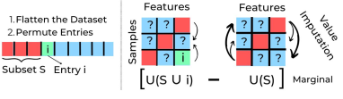
One idea to tackle the block valuation problem is to flatten the indices of blocks into one dimension and leverage 1D-Shapley to value each block. Specifically, we can reindex by . Note that this step discards the structural information contained in the two-dimensional indices. Then, one can utilize Eq. (1) to value each .
The second step of applying Eq. (1) requires calculating for any . Both and could correspond to a data fragment with samples differing in their feature space (see example in Figure 2); nevertheless, how to evaluate the utility of such a fragment is unclear. An ad hoc way of addressing this problem is to perform missing value imputation, e.g., filling out the missing values of a feature using the average of the feature values present.
In addition to the difficulty of evaluating the counterfactual, the symmetry axiom satisfied by 1D-Shapley no longer has the correct fairness interpretation when the input indices are flattened from 2D ones. In that case, , carry specific meanings entailed by the original 2D structure; e.g., some indices might correspond to temperature features, and others might correspond to humidity. Hence, the symmetry axiom that requires unchanged data values after permuting the data sources’ indices is not sensible and necessary, as the permutation might map the content of a data source from one meaning to an entirely different one.
We will use 1D-Shapley with missing value imputation as a baseline for our proposed approach. This simple baseline is still a useful benchmark to assess the extra (non-trivial) gains in different application scenarios that our approach can attain.
3.3 Our Approach: 2D-Shapley
Here, we will describe 2D-Shapley as a principled framework for valuing data blocks. We will emphasize how 2D-Shapley overcomes the challenges of the 1D-Shapley baseline in terms of (1) calculating the counterfactual, (2) framing the correct fairness principles, and then derive the representation of the data values based on the new counterfactual analysis and principle. At last, we will show efficient algorithms to compute 2D-Shapley.
3.3.1 Two-Dimensional Counterfactual Analysis
Given a two-dimensional utility function , we will define the marginal contribution of a block to the collection of blocks as
| (2) |
The rationality of the definition of can be shown by Figure 3. The area corresponding to can be viewed as the area , which subtracts these two areas of and , plus the area that is subtracted twice, the remaining area is shown in Figure 3 as “marginal”, which corresponds to the marginal influence of the block .

The unique advantage is that each individual utility is well-defined as it takes as input a collection of blocks within which the samples all share same feature space.
3.3.2 Axioms for Block Valuation
We start by redefining “dummy” for block valuation, where the underlying utility function is 2D.
Definition 3.1.
(2D-Dummy) We call a block a 2D-dummy under utility function if for all and ,
| (3) |
-dummy implies the canonical (one-dimensional) dummy mentioned in Section 2. Specifically, if sample is a sample dummy which satisfies and for like the dummy defined in 1D-Shapley, then Eq. (3) is satisfied with , and similarly, if feature is a feature dummy which satisfies and for , then Eq. (3) is also satisfied with . However, Eq. (3) can not imply sample is a sample dummy or feature is a feature dummy.
We first define the utility function set which contains all possible utility functions, and define a value function and denote the value of block as which is the th element in matrix . In order to build an equatable evaluation system, we provide the following axioms.
Axiom 1.
(2D-Linearity) For any two utility functions and any ,
| (4) |
Axiom 2.
(2D-Dummy) If the block is a dummy of which satisfies Eq. (3), then .
Axiom 3.
(2D-Symmetry) Let and be two permutations, then:
| (5) |
where for all ,
| (6) |
Axiom 4.
(2D-Efficiency) For every utility function ,
| (7) |
Let us discuss the rationality of the four axioms.
The 2D-linearity axiom is inherited from 1D-Shapley, which implies that the value of the -th block under the sum of two ML performance measures is the sum of the value under each performance measure.
The 2D-dummy axiom can be interpreted by taking . If a block has no contribution to the ML task, no matter what the situation (i.e., for any and ), then its value is zero.
In the 2D-symmetry axiom, the rows and columns are permuted independently. As a result, the entries from the same feature will always remain in the same column. The axiom state that such permutations would not change the value for individual data blocks, which is what we would expect in many ML applications. In Appendix A, we proved that Axiom 3 is implied by explanation here.
The 2D-efficiency axiom is inherited from 1D-Shapley, requiring that the sum of the values of all the data blocks equals the performance of the whole data set.
Based on the axioms, we provide a definition:
Definition 3.2.
The value with respect to the utility function is a two-dimensional Shapley value (2D-Shapley for short) if satisfies the 2d-linearity, 2d-dummy, 2d-symmetry and 2d-efficiency axioms, denoting as .
2D-Shapley can be seen as the two-dimensional extension of Shapley values, which inherits its advantage with a natural adaptation of the dummy and symmetry axiom to the two-dimensional utility function scenario.
3.3.3 Representation Theory
We will show that there exists an analytic and unique solution for 2D-Shapley.
Theorem 3.3.
(Representation Theory of 2D-Shapley) The has a unique solution:
| (8) |
where , ,
| (9) |
and defined in Eq. (2).
Theorem 3.3 indicates that is a weighted average of the two-dimensional counterfactual in Eq. (2). Theorem 3.3 is referred to as the representation theory of 2D-Shapley, because the proof procedure shows that has a basis expansion formulation (see Eq. (14) in Appendix B). To show the basis expansion, a series of basic utility functions in needs to be defined (e.g., Eq. (13)). Compared with the representation theory of 1D-Shapley by Roth (1988), one technical challenge is to define the basis and basic utility functions for the 2D case to handle the 2D counterfactual. Furthermore, the proof of the uniqueness of 2D-Shapley has to solve a complex high-dimensional linear system (see Eq. (18) in Appendix B). Our proof incorporates new techniques, unseen in the classic proof of 1D-Shapley, to deal with these unique technical challenges arising in the 2D context.
Moreover, the representation theory also implies that 2D-Shapley can be reduced to 1D-Shapley. The following corollary shows that summing up the block values over all rows gives 1D-Shapley of features, and summing up the block values over all columns gives 1D-Shapley of samples. Corollary 3.4 does not only indicate that the 2D-Shapley is a natural generalization of 1D-Shapley, but also is useful for discussing the experimental results of how 2D values can explain 1D values (see Subsection 4.1).
Corollary 3.4.
For any , let and , then
| (10) |
and
| (11) |
which are in the form of 1D-Shapley.
Finally, having the analytical expression Eq. (8) of 2D-Shapley at hand will provide us with great convenience in designing efficient algorithms.
3.3.4 Efficient Algorithm
The computational complexity of exactly calculating 2D-Shapley is exponential in due to the summation over all possible rows and columns. To overcome this challenge, we develop a Monte Carlo approach to approximating 2D-Shapley. The key idea is that 2D-Shapley can be rewritten as an expectation of the marginal contribution of to the blocks indexed by row indices before and column indices before over random permutations of rows and columns. As a result, we can approximate 2D-Shapley by taking an average over randomly sampled rows and columns. We also design the algorithm in ways that can reuse utility function evaluations across different permutations, which gives rise to significant efficiency gains. The full details of the algorithm design are provided in Appendix E, and the pseudo-code is shown in Algorithm 1.
Evaluating the utility function requires retraining a model. For small-scale datasets, it might be possible to evaluate the utility function within a reasonable time multiple times, but for large-scale datasets, even evaluating it once might require days to finish. This would deem our method impractical for any applications. Nonetheless, we can even obviate all model training to compute our values when using -nearest-neighbor (KNN) as a surrogate model. KNN-surrogate-based data valuation has shown great computational advantage while providing effective data quality identification (Jia et al., 2019a). In this work, we leverage a similar idea to reduce the computational complexity of 2D-Shapley for large models. First, let us observe from Eq. (8) and Corollary. D.1 that after rearranging inner terms, we have:
| (12) | ||||
where is a set of all permutations of , is a permutation of , and is a set of elements preceding in . The expression in the first bracket is the 1D marginal contribution of sample and is valid since both utilities are trained on same features, . Similarly, the second bracket also represents a valid 1D marginal contribution of the sample but with features . From this observation, we can apply the results of 1D-Shapley value approximated with nearest neighbors, , defined recursively in Theorem 1 (Jia et al., 2019a), and the 2D-Shapley under KNN surrogates can be therefore expressed as
This new formulation is efficient as it requires no more model training and removes the summing over all possible permutations of samples. We can further approximate the sum over all possible permutations over features with the average over sampled permutations. Our final complexity becomes , where is the number of sampled feature permutations, is the number of test points used for evaluating model performance, and are the cardinality of and respectively, and the pseudo-code for the overall KNN-based approximation is provided in Algorithm 2.
4 Experiments

This section covers the two general application scenarios of 2D-Shapley. (1) Cell valuation, where each cell in the training data matrix is considered a data source and receives a score indicating its contribution to a learning task performed on the matrix. We mainly demonstrate this application scenario’s benefits in fine-grained data debugging and interpreting canonical sample-wise or feature-wise data values. (2) Sub-matrix valuation, where a sub-matrix containing multiple cells is considered a data source and receives a joint score. This scenario is closely related to data marketplaces, where each entity provides a dataset that appears as a submatrix in the aggregated data. Details about datasets, models, implementations, and ablation studies on a budget of inserted outliers are provided in Appendix F.
4.1 Cell Valuation
Sanity check of cell-wise values.
We first check whether the cell-wise values produced by our method make sense via the data removal experiments commonly used in the data valuation literature. Specifically, we would expect that removing the cells with the highest values from the training set leads to the most significant performance degradation; conversely, removing the cells with the lowest values should barely affect the model performance. To evaluate the model performance after removal, we “remove” a cell by refilling its content with the average of all other cells on the same feature column. In the previous section, we present two algorithms to calculate 2D-Shapley. We will label the values obtained from the Monte Carlo-based method as 2D-Shapley-MC and the ones from the KNN-surrogate-based method as 2D-Shapley-KNN. 1D-Shapley and random removal are used as our baselines. In particular, 1D-Shapley is estimated by the permutation sampling described in (Jia et al., 2019b). For each baseline, we remove a number of cells at a time based on their sample-feature value ranking in either descending or ascending order; then, we train a model on the reduced dataset and evaluate the model performance.
As shown in Figure 4, when removing cells in ascending value order, 2D-Shapley can not only maintain the model performance but also improve it by at least for Census, Credit, and Breast Cancer datasets, whereas 1D-Shapley dips the model performance earlier than 2D-Shapley in all three datasets. Considering removal from the highest valued cells, we observe that 2D-Shapley can effectively detect contributing cells, and removing these cells causes the model performance to drop quickly. By contrast, removing cells according to 1D-Shapley is close to random removal. These results indicate that 2D-Shapley is more effective than 1D-Shapley at recognizing the contribution of cells and can better inform strategic data harnessing in ML.
Fine-Grained Outlier Localization.
Existing horizontal data valuation methods have demonstrated promising results in detecting abnormal samples (Ghorbani & Zou, 2019; Kwon & Zou, 2022; Wang & Jia, 2023) by finding lowest-valued samples. However, it is rarely the case that every cell in the sample is abnormal. For instance, a type of error in the Census data is “198x189x”, where the years of birth are wrongly specified; this error could appear on a single feature column and, at the same, only affects partial samples (or users) born in 198x. Existing horizontal valuation remains limited in localizing these erroneous entries.
To demonstrate the potential of 2D-Shapley in fine-grained entry-wise outlier detection, we first inject outlier cells into the clean dataset, Breast Cancer Dataset. Following a recent outlier generation technique in (Du et al., 2022), we inject low-probability-density values into the dataset as outlier cells. We explain the outlier injection method in detail in Appendix F.3. We randomly place outlier cells in (50 of total cells). Afterward, we compute 2D-Shapley-KNN for each cell in the dataset with inserted outliers, which are shown in Figure 10. Since we expect outliers not to be helpful for the model performance, the values for outlier cells should be low. Therefore, we sort the 2D-Shapley cell values in ascending order and prioritize human inspection towards the ones with the lowest values. We show the detection rate of the inserted outliers in Figure 5A). As we can see, with 2D-Shapley values, we can detect of inserted outliers within the first of all cells. By contrast, based on the values produced by 1D-Shapley, one would need over of cell inspection to screen out all the outlier cells.


We further examine a practical case of outliers caused by human errors, where the cells have been incorrectly typed, e.g., “18” became “81”. In the Census dataset, for the feature “Age”, we randomly swap 15 cells between “17” and “71”, “18” and “81”, “19” and “91”. Similarly, we sort the values of all cells in the dataset in ascending order. As we observe in Figure 5B), detection with 2D-Shapley outperforms 1D-Shapley. Particularly, with 2D-Shapley we can detect of added outliers with less than inspected cells while 1D-Shapley requires times as many cells to achieve a comparable rate. The 1D-Shapley and 2D-Shapley heatmaps are provided in Appendix. The results above demonstrate the effectiveness of 2D-Shapley in locating outlier cells in a dataset.
Enabling Interpretation of 1D Valuation Results.
Apart from outlier detection, 2D-Shapley also brings new insights into horizontal sample valuation or vertical feature valuation, which is referred to as 1D valuation. For instance, 1D sample valuation produces an importance score for each sample, but we lack a deeper understanding of why a sample receives a certain value. Recall Corollary 3.4 that the sum of 2D-Shapley over rows or columns gives 1D feature values and 1D sample values, respectively. Hence, 2D-Shapley allows one to interpret the 1D value of a sample by further breaking it down to contributions of different features in that sample. That is, 2D-Shapley gives insights into the relative importance of different features of a sample to the valuation result received by the sample. For example, in Figure 7A), we observe that two samples have similar 1D values and their cell values are also close. However, in Figure 7B), we observe a contrasting case, where although both samples have a close 1D value, their cell values are completely unrelated. More detailed results can be found in Appendix F.3.
4.2 Sub-matrix Valuation
We turn to the application of 2D-Shapley to inform dataset pricing in the data marketplace. 2D-Shapley enables a principled method to value fragmented data sources as illustrated in Figure 1(c), where each source is a sub-matrix in the aggregated training data matrix. A reasonable measure of a source’s value should reflect its usefulness for ML. Hence, to verify the significance of the resulting values for sub-matrix valuation, we measure the model performance trained on a source and examine the correlation between its value and the performance. For this experiment, we use the Credit Dataset with sources contributing fragmented data and consider multiple random splits of the dataset. The results are provided in Figure 6, where each line corresponds to a different split of the aggregate data into individual sources. Figure 6 shows that with the increasing model performance trained on the block, its corresponding 2D-Shapley block value also increases.
5 Conclusion
This work aims to set the theoretical foundation for more realistic data valuation application scenarios. In particular, we investigate the block valuation problem and present 2D-Shapley, a new data value notion that is suitable to solve this problem. 2D-Shapley empowers a range of new use cases, such as informing the pricing of fragmented data, strategic data selection on a fine-grained scale, and interpreting 1D valuation results. Our work opens up many new venues for future investigation. First, we can immediately adapt our proof technique to prove a two-dimensional generalization of other typical data value notions (Kwon & Zou, 2022; Wang & Jia, 2023). Second, it is interesting to build upon our framework to evaluate irregular-shaped data sources (Fang et al., 2019) and incorporate label information for joint valuation in a principled way.
Acknowledgements
Xiangyu Chang’s work was partly supported by the National Natural Science Foundation for Outstanding Young Scholars of China under Grant 72122018 and partly by the Natural Science Foundation of Shaanxi Province under Grant 2021JC-01. Xi Chen would like to thank the support from NSF via the Grant IIS-1845444. RJ and the ReDS lab would like to thank the support from NSF via the Grant OAC-2239622.
References
- Covert et al. (2020) Covert, I., Lundberg, S. M., and Lee, S.-I. Understanding global feature contributions with additive importance measures. Advances in Neural Information Processing Systems, 33:17212–17223, 2020.
- Du et al. (2022) Du, X., Wang, Z., Cai, M., and Li, Y. Vos: Learning what you don’t know by virtual outlier synthesis. arXiv preprint arXiv:2202.01197, 2022.
- Dua & Graff (2017) Dua, D. and Graff, C. UCI machine learning repository, 2017. URL http://archive.ics.uci.edu/ml.
- Fang et al. (2019) Fang, F., Lan, W., Tong, J., and Shao, J. Model averaging for prediction with fragmentary data. Journal of Business & Economic Statistics, 37(3):517–527, 2019.
- Ghorbani & Zou (2019) Ghorbani, A. and Zou, J. Data shapley: Equitable valuation of data for machine learning. In International Conference on Machine Learning, pp. 2242–2251. PMLR, 2019.
- Jia et al. (2019a) Jia, R., Dao, D., Wang, B., Hubis, F. A., Gürel, N. M., Li, B., Zhang, C., Spanos, C. J., and Song, D. Efficient task-specific data valuation for nearest neighbor algorithms. Proceedings of the VLDB Endowment, 12(11):1610–1623, 2019a.
- Jia et al. (2019b) Jia, R., Dao, D., Wang, B., Hubis, F. A., Hynes, N., Gürel, N. M., Li, B., Zhang, C., Song, D., and Spanos, C. J. Towards efficient data valuation based on the Shapley value. In The 22nd International Conference on Artificial Intelligence and Statistics, pp. 1167–1176. PMLR, 2019b.
- Just et al. (2023) Just, H. A., Kang, F., Wang, J. T., Zeng, Y., Ko, M., Jin, M., and Jia, R. Lava: Data valuation without pre-specified learning algorithms. In International Conference on Learning Representations, 2023.
- Karlaš et al. (2022) Karlaš, B., Dao, D., Interlandi, M., Li, B., Schelter, S., Wu, W., and Zhang, C. Data debugging with shapley importance over end-to-end machine learning pipelines. arXiv preprint arXiv:2204.11131, 2022.
- Kwon & Zou (2022) Kwon, Y. and Zou, J. Beta Shapley: a unified and noise-reduced data valuation framework for machine learning. In International Conference on Artificial Intelligence and Statistics, pp. 8780–8802. PMLR, 2022.
- Lin et al. (2022) Lin, J., Zhang, A., Lécuyer, M., Li, J., Panda, A., and Sen, S. Measuring the effect of training data on deep learning predictions via randomized experiments. In International Conference on Machine Learning, pp. 13468–13504. PMLR, 2022.
- Lundberg & Lee (2017) Lundberg, S. M. and Lee, S.-I. A unified approach to interpreting model predictions. Advances in Neural Information Processing Systems, 30:4768–4777, 2017.
- Roth (1988) Roth, A. E. The Shapley value: essays in honor of Lloyd S. Shapley. Cambridge University Press, 1988.
- Shapley (1953) Shapley, L. S. A value for n-person games. Contributions to the Theory of Games, 2(28):307–317, 1953.
- Shapley (1997) Shapley, L. S. A value for n-person games. Classics in game theory, 69, 1997.
- Strumbelj & Kononenko (2010) Strumbelj, E. and Kononenko, I. An efficient explanation of individual classifications using game theory. Journal of Machine Learning Research, 11:1–18, 2010.
- Tang et al. (2021) Tang, S., Ghorbani, A., Yamashita, R., Rehman, S., Dunnmon, J. A., Zou, J., and Rubin, D. L. Data valuation for medical imaging using Shapley value and application to a large-scale chest X-ray dataset. Scientific Reports, 11(1):1–9, 2021.
- Tay et al. (2022) Tay, S. S., Xu, X., Foo, C. S., and Low, B. K. H. Incentivizing collaboration in machine learning via synthetic data rewards. In Proceedings of the AAAI Conference on Artificial Intelligence, volume 36, pp. 9448–9456, 2022.
- Wang & Jia (2023) Wang, J. T. and Jia, R. A robust data valuation framework for machine learning. In International Conference on Artificial Intelligence and Statistics. PMLR, 2023.
- Wang & Jia (2022) Wang, T. and Jia, R. Data banzhaf: A data valuation framework with maximal robustness to learning stochasticity. arXiv preprint arXiv:2205.15466, 2022.
- Wu et al. (2022a) Wu, M., Jia, R., Huang, W., Chang, X., et al. Robust data valuation via variance reduced data shapley. arXiv preprint arXiv:2210.16835, 2022a.
- Wu et al. (2022b) Wu, Z., Shu, Y., and Low, B. K. H. Davinz: Data valuation using deep neural networks at initialization. In International Conference on Machine Learning, pp. 24150–24176. PMLR, 2022b.
- Yan & Procaccia (2021) Yan, T. and Procaccia, A. D. If you like shapley then you’ll love the core. In Proceedings of the AAAI Conference on Artificial Intelligence, volume 35, pp. 5751–5759, 2021.
- Yona et al. (2021) Yona, G., Ghorbani, A., and Zou, J. Who’s responsible? jointly quantifying the contribution of the learning algorithm and data. In Proceedings of the 2021 AAAI/ACM Conference on AI, Ethics, and Society, pp. 1034–1041, 2021.
- Yoon et al. (2020) Yoon, J., Arik, S., and Pfister, T. Data valuation using reinforcement learning. In International Conference on Machine Learning, pp. 10842–10851. PMLR, 2020.
Appendix A Proof of the fact that Axiom 3 is implied by its explanation
The explanation above is: for , , if for any and , , and for any and , , then .
For the proof, we prove in three steps that the explanation is equivalent to Axiom 3. Note that we should assume Axiom 1, 2 and 4 already exist. For simplicity, we use the lowercase letter to denote the cardinality of a set, for example, .
We want to prove the following proposition.
Proof.
For the direction that Axiom 3 is implied by its explanation, we prove in three steps.
-
•
Step 1: Define a utility function :
(13) For fixed , and , and for all , . It leads to the conclusion that according to the explanation.
For , (or , ) and , , (, ,) . (.) It leads to the conclusion that , (, ) according to Axiom 2.
In summary, we have conclusion that the values s are the same when , and otherwise zero. According to Axiom 4,
then , where .
-
•
Step 2: We have to prove a lemma which shows another formation of a utility by using defined above.
Lemma A.2.
where .
Proof.
We can directly verify the lemma.
∎
-
•
Step 3: Combine the first two steps, and by Axiom 1,
Let be two permutations on and respectively, then
For another direction that Axiom 3 implies its explanation, since we already assume Axiom 1, 2, 3 and 4 hold, then we have the formula of 2D-Shapley, that is, Eq. (21). Clearly, we can see the numerator is always the same for both and under the same and , hence .
∎
Appendix B Proof of the representation theory of 2D-Shapley
In this section, we will justify the representation theory by a number of proposed lemmas. The proof process is to add the axioms one by one and try to show what each axiom does for 2D-Shapley. We add linearity and dummy axioms first to get a sum of weighted marginals.
Lemma B.1.
Proof.
For any ,
| (14) |
where
By the 2d-linearity axiom,
Now define another utility function :
For any and , we can check that block is a dummy for , then by the 2d-dummy axiom, . Especially, let and any fixed , we have:
For inductive purposes, assume it has been shown that for fixed and every with . (The case has been proved.) Now take fixed with , then
Therefore, for all and fixed with and . Similarly, we have another conclusion that for fixed and all with and by simply defining another similar utility function and repeat the process above again.
Using the results above,
For simplicity, denote as , then
Consider the utility function ,
and we can check that is a dummy for , and . Hence
∎
Next, add the 2d-symmetry axiom to Lemma B.1 and we make the conclusion that is only related to the cardinality of and , which is not associated with the name of the blocks.
Lemma B.2.
Assume Lemma B.1 holds. If also satisfies the 2d-symmetry axiom, then
where is some common value for , and , .
Proof.
Define a utility :
-
1.
For and , let , and , be any two coalitions where and with and respectively. Consider two permutation and which satisfy and . Then,
where the central equality is a consequence of the 2d-symmetry axiom.
-
2.
For distinct and , let and , and the permutations respectively interchange and while leaving other elements fixed. Then,
where the central equality is a consequence of the 2d-symmetry axiom. Combining with the previous result in Step 1, we find that for every and , there is a such that for every and , and with , .
-
3.
Similarly, by using different utility functions, we can find for :
-
•
a such that for and ,
-
•
a such that for and ,
-
•
a such that for and ,
-
•
a such that , for and ,
-
•
a such that ,
-
•
a such that which makes the sum of all the weights equals to 1.
-
•
∎
Finally add the 2d-efficiency axiom and obtain the uniqueness of 2D-Shapley.
Lemma B.3.
Proof.
Now, let’s prove Theorem 3.3.
Proof of Theorem 3.3.
By Lemma B.2,
By Lemma B.1 and Lemma B.3, we have the following equations:
| (17) | ||||
Actually, we can omit the first equation and the conditions are:
| (18) | ||||
Hence, we have variables and equations.
Convert the Eq. (18) to matrix equations in the form of
where
and
| (20) |
where
And
For example, if , then
Convert to by using the elementary column and row transformation,
According to the property of the elementary row and column transformation,
Consider equation
and the solution is only , hence
Appendix C Proof of Corollary 3.4
Appendix D Permutation-based 2D-Shapley Formulation
To compute 2D-Shapley more efficient, we propose the following corollary.
Corollary D.1.
Eq. (8) has an equivalent form as follows:
| (21) |
or
| (22) |
where denotes a set of all permutations of and a set of all elements of that precede in the permutation .
The formulation in Eq. (21) is a simple derivation from Eq. (8) that sums marginal contributions over all subsets. Whereas, the second formulation in Eq. (22) sums over all sample and feature permutations, and the marginal contribution of block is weighted by a coefficient that measures all orderings of samples appearing before and after sample and all orderings of features appearing before and after feature . This corollary gives a simple expression of 2D-Shapley. Using this equivalent formulation, we can design efficient algorithms for 2D-Shapley implementation.
Appendix E Algorithm Details
Here, we explain the implementation of algorithms and explore ways to achieve efficient computation.
E.1 Saving Computation in 2D-Shapley-MC
First, we focus on 2D-Shapley-MC. Apart from Monte Carlo sampling on both sample and feature permutations to reduce complexity, we also reduce the number of model training to a single time for each counterfactual evaluation as opposed to , which is derived in Eq. 2. Let us observe that in the marginal contribution equation, we have utility terms, but actually, of them are already computed, which we can reuse them. We take a pair as an example. For the marginal contribution of , we have 4 utility terms to compute: . However, we notice that was already computed for a pair , for a pair , and for . Therefore, by saving these evaluations, we can reduce the total number of model training by . Saving all model evaluations for every block might overflow the memory. However, we only need to save the utilities of the previous and current rows (columns) if we are looping horizontally downwards (vertically rightwards), which promotes efficient memory usage. Additionally, our algorithm can be parallelized. In particular, every permutation can be computed independently and combined at the last stage, which is the “while loop” in Algorithm 1.
E.2 Limitations of 2D-Shapley-MC and Possible Improvements
One limitation of the Monte Carlo method is time complexity which scales with the number of rows and columns in an aggregate data matrix. To improve the efficiency of 2D-Shapley-MC, we can reduce the burden on model retraining of 2D-Shapley-MC to lower the computation cost. For example, there exist highly efficient methods for model re-training, such as FFCV [1,2], which has been applied in Datamodels [3] and can significantly reduce computation complexity. Another limitation is that 2D-Shapley-MC relies on the performance scores associated with models trained on different subsets to determine the cell values. However, these values are susceptible to noise due to training stochasticity when the learning algorithm is randomized (e.g., SGD) (Wang & Jia, 2022). To overcome these limitations, we proposed an efficient, nearest-neighbor-based method, 2D-Shapley-KNN, which involves no model training and only requires sorting data. With this method, we also avoid the problem of model training stochasticity, which 2D-Shapley-MC is facing with. Another advantage of 2D-Shapley-KNN is that it has an explicit formulation for sample values and only requires permuting over features. This method not only beats 2D-Shapley-MC by an order of magnitude in terms of computational efficiency but is straightforward to compute and only requires CPU resources.
E.3 Saving Computation in 2D-Shapley-KNN
Apart from removing the dependency on the sample permutations and all model training, 2D-Shapley-KNN can further be reduced in computation. Similar to the 2D-Shapley-MC, we here also save the utility terms, as shown in Algorithm 2. For each pair , we need to compute and . However, the second term was already calculated for the previous feature in prior to . Thus, we can reduce the total number of evaluations by .
Input: Training Set , Learning Algorithm , Test Set , Utility Function .
Output: Sample-Feature 2D Shapley Values .
Ensure: , ; .
while not converged do
Input: Training Set , Test Set , Top .
Output: Sample-Feature 2D Shapley Values .
Ensure: , ; .
while not converged do
E.4 Actual Runtime Complexity
Time complexity is an important aspect when evaluating the efficiency of algorithms. In our case, we focus on determining the runtime of our methods for different number of cell valuations on the Census dataset until the values’ convergence is achieved. While computing the runtime for the exact 2D Shapley runtime, we encounter a challenge due to the exponential growth of permutations with the cell size, making exact 2D Shapley intractable to compute. To address this, we benchmark the exact 2D Shapley runtime, by measuring the runtime for a single permutation and scale it by the total number of permutations needed for the exact 2D Shapley. As we observe in Table 1, 2D-Shapley-KNN, exhibits exceptional efficiency compared to 2D-Shapley-MC across various cell valuations on the Census dataset. At 1,000 cells valuation, 2D-Shapley-KNN was at least 25 times faster than 2D-Shapley-MC, showcasing a substantial advantage. Furthermore, as the number of cells increased to 100,000, 2D-Shapley-KNN demonstrates a remarkable speed advantage, being approximately 300 times faster than 2D-Shapley-MC. These findings clearly establish an advantage of 2D-Shapley-KNN over 2D-Shapley-MC in terms of runtime efficiency. Moreover, we observe that both 2D-Shapley-KNN and 2D-Shapley-MC outperform the exact 2D Shapley method in terms of runtime. These results highlight the effectiveness and practicality of our approach for computing 2D-Shapley in real-world cases.
| Method | 1K | 5K | 10K | 20K | 50K | 100K | ||
|---|---|---|---|---|---|---|---|---|
|
1.5E+301s | 2.0E+1505s | 2.8E+3010s | 5.6E+6020s | 4.4E+15051s | 1.4E+30103s | ||
| 2D-Shapley-MC | 280s | 1,661s | 3,127s | 9,258s | 17,786s | 26,209s | ||
| 2D-Shapley-KNN | 11s | 25s | 37s | 44s | 53s | 88s |
Appendix F Implementation Details & Results
F.1 Details on Datasets and Models
For our experiments, we use the following datasets from Machine Learning Repository (Dua & Graff, 2017):
| Dataset | Training Data | Test Data | Features |
|---|---|---|---|
| Census Income | 32561 | 16281 | 14 |
| Default of Credit Card Clients | 18000 | 12000 | 24 |
| Heart Failure | 512 | 513 | 13 |
| Breast Cancer Wisconsin (Original) | 242 | 241 | 10 |
| Wine Dataset | 106 | 72 | 13 |
In Breast Cancer Wisconsin dataset, we removed “ID number” from the list of features as it was irrelevant for model training.
For methods requiring model training, 1D-Shapley, Random, and 2D-Shapley-MC, we implemented a decision tree classifier on all of them.
Empirically, we verified that for each of the method, the cell values converge within permutations and that is the number we decide to use to run these methods.
Due to varying sizes of each dataset with different number of features, we set a different number of cells to be removed at a time. For bigger datasets, Census Income and Credit Default, we remove ten cells at a time, and for a smaller dataset, Breast Cancer, we remove one cell at a time.
F.2 Additional Results on Sanity check of cell-wise values experiment

We provide results on additional datasets, Heart Failure and Wine Dataset, to demonstrate the effectiveness of 2D-Shapley in cell-wise valuation. We additionally include the 2D LOO baseline for comparison. As we can observe in Figure 8, 2D LOO performance is comparable to or worse than the Random baseline. One of the main reasons is that 2D LOO only valuates a cell’s contribution when all other cells are present. This means that after the sequential removal of some cells, the values obtained from 2D LOO may no longer accurately represent the importance of the cells. In contrast, our method computes a cell’s value by averaging its contribution over various sample and feature subset sizes, which ensures our cell values are informative even after the sequential removal of a certain amount of cells, thereby addressing the shortcomings of 2D LOO and leading to improved performance in cell-wise valuation.
F.3 Additional Details and Results on Fine-Grained Outlier Localization experiment
F.3.1 Outlier Value Generation
Our outlier generation technique is inspired by (Du et al., 2022). Specifically, for a random cell with a sample index and a feature index , we generate an outlier value based on its feature . We first recreate a distribution of the feature and then sample a value from a low-probability-density region, below in our experiment.
F.3.2 Heatmaps Comparison
To better understand the detection rate of outlier values, we visualize them through a heatmap. In Figure 9, we provide a 2D-Shapley heatmap of the original dataset before outlier injection and compare with a 2D-Shapley heatmap in Figure 10 after injecting outliers. Due to dimensional reasons, we transpose the heatmap, where the rows represent features and the columns denote the samples.
We observe through the breast cancer dataset that the cells with injected outliers have changed their values and lie mostly in the lower range of 2D-Shapley values. However, we can also notice that other cells are also affected by the outliers and the overall range of values has increased in both directions.


In addition, we present a heatmap with injected outliers generated by 1D-Shapley to provide insights into the 1D-Shapley detection performance, which we show in Figure 5A). As we can observe the 1D-Shapley heatmap in Figure 11, the values of injected outliers are scattered which explains why the detection rate by 1D-Shapley was suboptimal.
F.3.3 Ablation Study on the Budget of Inserted Outliers
In Figure 5A), we injected outlier values to of total cells. Here, we explore whether our 2D-Shapley method can still detect outliers on various different amount of outliers. Thus, we randomly inject of outlier values to the original breast cancer dataset and plot the detection rate.

As we observe in Figure 12, the detection rate of outliers is very high within the first inspected cells for every outlier injection rate. Further, we observe that with more outliers added to the dataset, our detection rate slightly decreases. It is indeed reasonable, since as we inject more outliers in the dataset, the less uncommon these outliers are.
F.4 Additional Details on Sub-matrix Valuation experiment
For the plots in Figure 6, we have randomly split the Credit Default dataset into blocks. One of the random split is pictured in Figure 13. We randomly moved the horizontal and vertical lines and permuted separately rows and columns to create different possibilities for block splits.

F.5 Hardware
In this work, we used an 8-Core Intel Xeon Processor E5-2620 v4 @ 2.20Ghz CPU server as a hardware platform.
F.6 Code
The code repository is available via this link https://github.com/ruoxi-jia-group/2dshapley.